Tag Archives: level of detail expressions

TRIMMEAN() in Tableau

Excel’s TRIMMEAN() function can be quite useful at removing outliers, essentially it removes the top and bottom Nth percent of values and then computes the mean of the rest. Here’s the equivalent formula in Tableau that in Superstore Sales computes the TRIMMEAN() of sales at the customer level removing the top and bottom 5th percentile of customers when used with the AVG() aggregation:

{FIXED [Customer Name]: SUM(
    IF {FIXED [Customer Name] : SUM([Sales])} < 
    {FIXED : PERCENTILE({FIXED [Customer Name] : SUM([Sales])}, .95)}
    AND {FIXED [Customer Name] : SUM([Sales])} > 
    {FIXED : PERCENTILE({FIXED [Customer Name] : SUM([Sales])}, .05)} THEN
       [Sales]
    END)
}

Read on for how to build and validate your own TRIMMEAN() equivalent in Tableau.

When building out calculations in Tableau I try to let Tableau do as much of the computation as possible for both the calculations and the validation, so I’m typing as little as I can. Starting with Superstore, let’s identify the top and bottom 5th percentiles, here’s a view using a reference distribution:

Screen Shot 2016-07-12 at 3.57.38 PM

Now we know what we’re going to have to remove. The next step is to duplicate this worksheet as a crosstab, then build out calcs that can return the 5th and 95th percentiles of Sales at the Customer Name level. While this can be done with table calculations (here’s an example from the Tableau forums) I’m going to use FIXED Level of Detail Expressions so I’ve got a dimension I can use, so for example I could compare the trimmed group to the non-trimmed group. Here’s the 95th percentile Level of Detail Expression:

{FIXED : PERCENTILE({FIXED [Customer Name] : SUM([Sales])}, .95)}

The inner LOD is calculating the sales at the Customer level, then the outer LOD is returning the 95th percentile as a record level value. Here’s the two calcs which have values that compare to the reference lines above:

Screen Shot 2016-07-12 at 4.03.46 PM

The next step is to filter out the values outside of the desired range, here’s the TRIMMEAN Filter formula:

{FIXED [Customer Name] : SUM([Sales])} < 
    {FIXED : PERCENTILE({FIXED [Customer Name] : SUM([Sales])}, .95)}
AND {FIXED [Customer Name] : SUM([Sales])} > 
    {FIXED : PERCENTILE({FIXED [Customer Name] : SUM([Sales])}, .05)}

This uses the 5th and 95th percentile formulas and only returns True when the Customer level sales is less than the 95th percentile or greater than the 5th percentile, we can visually validate it by dropping it on the Color Shelf:
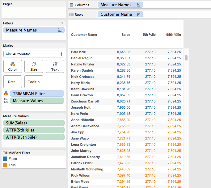
Screen Shot 2016-07-12 at 4.06.37 PM

Now that we have this the next step is to calculate what the trimmed mean would be. Again, we can use a view with a reference line, this time it’s been filtered using the TRIMMEAN Filter calc and the reference line is an average:

Screen Shot 2016-07-12 at 4.08.16 PM

Now we can embed the TRIMMEAN Filter formula inside an IF/THEN statement to only return the sales for the filtered values, this is the Trimmed Sales calc:

IF {FIXED [Customer Name] : SUM([Sales])} < 
   {FIXED : PERCENTILE({FIXED [Customer Name] : SUM([Sales])}, .95)}
AND {FIXED [Customer Name] : SUM([Sales])} > 
   {FIXED : PERCENTILE({FIXED [Customer Name] : SUM([Sales])}, .05)} THEN
   [Sales]
END

And here it is in the workout view, only returning the sales for the trimmed customers:
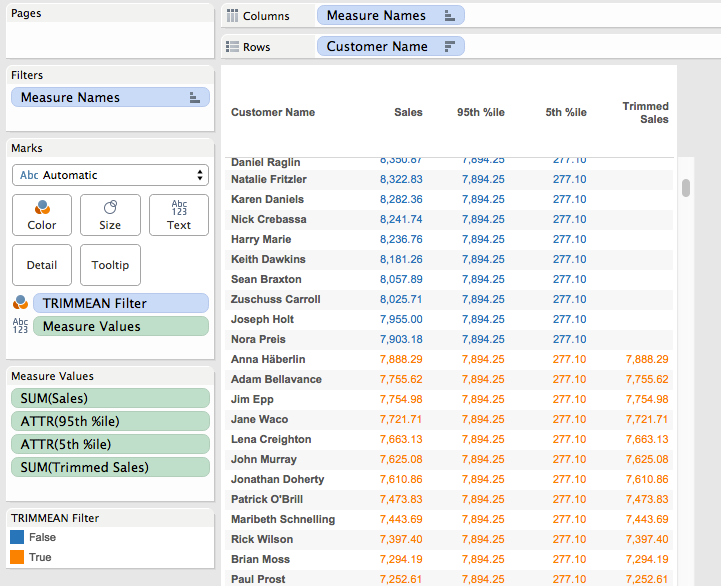
Screen Shot 2016-07-12 at 4.15.36 PM

Now that we have the trimmed sales there are two ways we can go. If we want the trimmed mean without the Customer Name in the Level of Detail then we can validate that in our workout view by using Tableau’s two-pass Grand Totals to get the average of the customer-level trimmed sales. This was created by:

  1. Removing the TRIMMEAN Filter pill from Colors (this increases the vizLOD and is no longer necessary).
  2. Clicking on the Analytics tab.
  3. Dragging out a Column Grand Total.
  4. Right-clicking the SUM(Trimmed Sales) pill on Measure Values and setting Total Using->Average.

Scrolling down to the bottom we can see that the overall trimmed mean matches of 2,600.79 matches the one from the reference line.

Screen Shot 2016-07-12 at 4.20.33 PM

Note that we could have used the Summary Card instead, however using the Grand Total lets us see exact values.

There’s a problem, though, if we use the Trimmed Sales all on its own in a view it breaks, whether using SUM() or AVG():
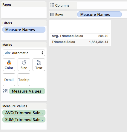
Screen Shot 2016-07-12 at 4.25.49 PM

The reason why is that the Trimmed Sales is a record level value and Superstore is at the level of detail of individual order items, but we’re trying to compute the trimmed mean across Customer Names. For the true trimmed mean in this case we need to aggregate this trimmed sales to the Customer Name like we did in the workout view, here’s the Trimmed Sales (Customer Level) formula that uses the Trimmed Sales and wraps that in an LOD to get the Customer Level sales:

{FIXED [Customer Name]: SUM(
    IF {FIXED [Customer Name] : SUM([Sales])} < 
    {FIXED : PERCENTILE({FIXED [Customer Name] : SUM([Sales])}, .95)}
    AND {FIXED [Customer Name] : SUM([Sales])} > 
    {FIXED : PERCENTILE({FIXED [Customer Name] : SUM([Sales])}, .05)} THEN
       [Sales]
    END)
}

This returns the same results in the workout view:

Screen Shot 2016-07-12 at 4.31.49 PM

And works all on its own in a view:

Screen Shot 2016-07-12 at 4.32.32 PM

Now this is a case where the FIXED level of detail expression is returning different results depending on the level of detail of the view, if we want it to return the same result then we can wrap all that in one more LOD expression, this is the TRIMMEAN Fixed calculation:

{FIXED : AVG(
    {FIXED [Customer Name]: SUM(
        IF {FIXED [Customer Name] : SUM([Sales])} < 
        {FIXED : PERCENTILE({FIXED [Customer Name] : SUM([Sales])}, .95)}
        AND {FIXED [Customer Name] : SUM([Sales])} > 
        {FIXED : PERCENTILE({FIXED [Customer Name] : SUM([Sales])}, .05)} THEN
            [Sales]
        END)
    })
}

And here it is in the workout view and a view without any dimensions:

Screen Shot 2016-07-12 at 4.34.36 PM

Screen Shot 2016-07-12 at 4.35.35 PM


Final Comments

This is a good (and bad) example of how Tableau is different from Excel. In one bad sense note that I didn’t parameterize the percentage for the trimmed mean, this is because in Tableau it would require two parameters because we can’t put calculations as the arguments to the PERCENTILE() function. In another bad sense the calculation requires understanding Level of Detail expressions and is not wrapped into a simple formula. On the other hand we’ve got very precise control over what the calculation is computing over with those Level of Detail expressions and aren’t just limited to doing trimmed means, we could do trimmed medians, get the Nth percentile of the trimmed values, etc.

Here’s the trimmed mean workbook on Tableau Public.

Sorting a Dimension by Two Values At Once

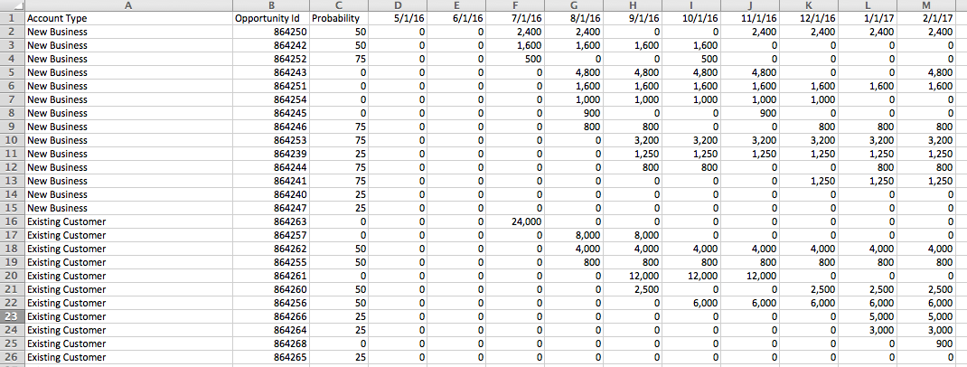
I recently got a question via email about how to sort a view by two different criteria at the same time. Here’s an Excel table of opportunities where for each month and Opportunity ID there’s a forecast of size of opportunity:

Screen Shot 2016-06-30 at 2.12.45 PM

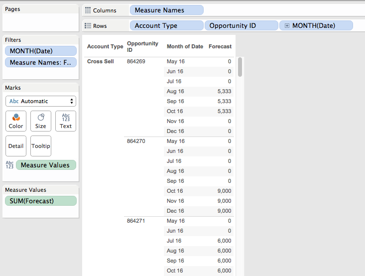
The goal here is to sort the opportunities within each account type by the nearest (by month) and biggest opportunities (by Forecast size) first, so it looks more like this in Tableau:

Screen Shot 2016-06-30 at 2.13.38 PM

Now with that data in Excel arranged in a tabular form I can sort on December, then November, then October, and so on, and get the desired sort:

Screen Shot 2016-06-30 at 2.14.29 PM

But in Tableau I can’t do that, if I try to work with the data in that “wide” format with a column for each month it just won’t work. If I use Tableau’s pivot feature to make the data “tall” with a record for each Opportunity ID and Month then I still run into problems. I want to sort the opportunities by each month and by Forecast but when I try to sort the Opportunity ID dimension I can’t get it to work, it only sorts by a single month’s values, so in the view below Opportunity ID 864280 should be the first new one for August since:

Screen Shot 2016-06-30 at 2.15.31 PM

The Excel way isn’t good because each month I have to manually re-sort the data. And in Tableau it just seems impossible to get the right sort because it looks like we need to sort in two different directions at once (get the earliest non-zero month for each opportunity, and then sort up and down the opportunities in each account type), and Tableau only lets us sort on one thing at a time. However, it is possible – read on for how to get this kind of sort in Tableau and maybe learn a few math tricks!

Part of how this kind of problem can be more challenging is the way the problem (and data) is initially presented to us. When we see the data in the crosstab form in Tableau the *appearance* is that we need to sort in two different directions. In fact, we really only need to sort in one direction based on the forecast value in the first month for each opportunity, so in the view below we’d want Opportunity ID 864271 to be the first one sorted because it’s from July 2016.

Screen Shot 2016-06-30 at 2.16.45 PM

Each opportunity row in the view needs to be sorted within the account type by the first (earliest) month where there is a non-zero forecast and then by the value of Forecast in descending order for that month.

The key to sorting headers and panes in Tableau is that it’s done using the discrete (blue) pills on Rows or Columns from left to right. So the left-most discrete (blue) pill headers are sorted, then the 2nd discrete pill’s headers are sorted, and so on. For discrete dimensions from a primary source we can sort by a measure, use the default alphanumeric sort, or a manually, otherwise any discrete pills are by default alphanumerically sorted or manually sorted.

Therefore in this case I knew I needed to either return a measure that could sort some dimension (like the Opportunity ID) or return a discrete dimension value that with the default alphanumerical sort would work right. Note that filtering wouldn’t work here because the goal is to show a sorted crosstab.

The next part of working out the solution is how to structure this value for sorting. I’ve done some multi-level sorting in the past where I needed a nested sort of single dimension by two different criteria, and a common construct is a number of the form X.Y where the integer portion X is from one criteria and the decimal portion N is from the other criteria. So with the default alphanumerical sort 1.2 comes before 1.3 comes before 2.1 etc.

So for the integer part of the sort I need to convert the date for each opportunity into a number where the Forecast is greater than 0. The Date Number (temp) calc has the formula:

IF [Forecast] > 0 THEN
    INT([Date])
END

Screen Shot 2016-06-30 at 2.17.34 PM

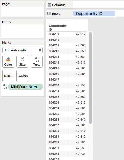
This convers the date into an integer, in this case the number of days since 1/1/1900. To get the first (earliest) month for each opportunity then all I need to do is aggregate it with MIN() at the level of Opportunity ID:

Screen Shot 2016-06-30 at 2.18.01 PM

Ultimately, this is is what we’re going to do to get that pill sort of Opportunity ID’s in the final view.

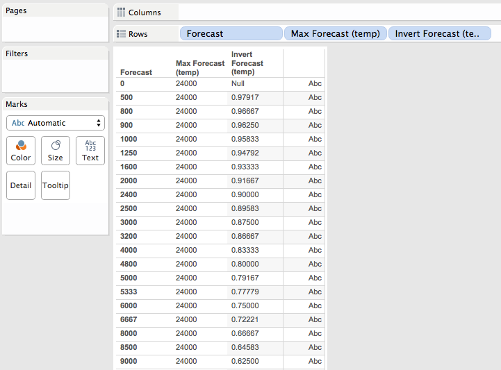
For the decimal part of the sort I needed a number where the smallest numbers reflected the largest values, and it needed a value between 0 and 0.999999 (it can’t be a whole value of 1 because that would affect the integer sort). A way to turn a set of positive numbers into decimal numbers between 0 and 1 is to do X/(max X). In this case X is the Forecast, so to get the max X in the data I used the Level of Detail Expression, here’s the Max Forecast (temp) formula:

{FIXED : MAX([Forecast])}

Screen Shot 2016-06-30 at 2.18.35 PM

Now if I do [Forecast]/MAX([Forecast]) that’s going to return a number between 0 and 1 that preserves the original ordering of values, i.e. bigger values of Forecast are closer to 1. So to invert that I used use 1 – X/(max X). So if (max X) is 10 and X is 9, then the result of (1 – 9/10) is 0.1, while if X is 2 then the result of (1- 2/10) is 0.8, a bigger number.

We avoid results of 1 that could affect the sort by skipping values of where the Forecast is 0, here’s the Invert Forecast (temp) formula:

IF [Forecast] > 0 THEN
    1-[Forecast]/[LOD Max Forecast Value]
END

Screen Shot 2016-06-30 at 2.19.19 PM

I could have avoided the LOD expression for the max value by just setting a gigantically huge number, however past experience with foreign currencies has shown me that whatever huge number I can imagine is likely to be smaller than reality so I chose to make sure that the value is coming from the data

With all the values worked out I could now put everything together into a single calculation, this is the Sort calc that returns record-level values:

IF [Forecast] > 0 THEN
    INT([Date])
    + (1-[Forecast]/{FIXED : MAX([Forecast])})
//Forecast is 0, return a really big number that will be put at the end of the sort
ELSE
    999999
END

Screen Shot 2016-06-30 at 2.20.09 PM

This calc returns the numbers as record level values.

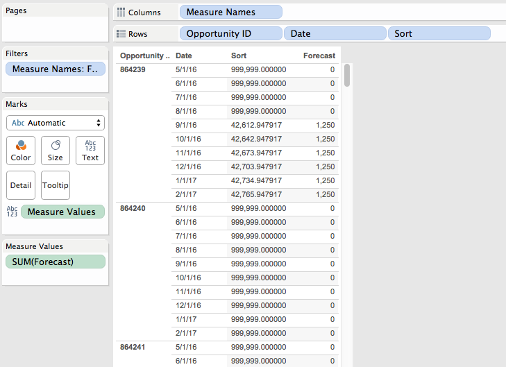
To show how the sort works out I set up this view where the Sort calc is used as the leftmost discrete dimension to show what gets sorted first, with the bar chart we can quickly visually verify that the dates are sorted with earliest months first and then by the Forecast within each month:

Screen Shot 2016-06-30 at 2.20.41 PM

Note that there’s a different value for each Opportunity ID/month combination, when what we really want is that single minimum value for each Opportunity ID/month. So we need to aggregate the Sort measure with MIN() at the level of detail of Opportunity ID, and we can do just that using a pill sort on the Opportunity ID dimension:

Screen Shot 2016-06-30 at 2.21.14 PM

Now we can arrange pills to build the original crosstab view and have the desired sort:

Screen Shot 2016-06-30 at 2.13.38 PM

And as the data updates the sort will automatically work, in this case I’ve added January 2017 to the data:

Screen Shot 2016-06-30 at 2.22.37 PM

Conclusion

The following bits of Tableau knowledge were necessary to get the desired results:

  • How Tableau sorts views using discrete pills.
  • How Tableau’s pill sorts work.
  • A tiny bit of Level of Detail Expression building.

And then the following math tricks were used:

  • Combining two different numbers into one using an integer number for one value and a decimal number for the second value.
  • Making positive numbers into a range of 0-1 using X/(max X). A different formula would be needed if there were negative numbers and/or the desired range was different.
  • Inverting ranges to make big numbers small and small numbers big using 1 – X/(max X)

FYI if LOD expressions are not available in your particular data source then you could use a table calculation, a data blend, or just manually enter your equivalent of the Max Forecast value. I set up a table calculation version as well in the Sorting by Two Values Tableau Public workbook.