Tag Archives: table calculations

Text Wrapping within Tableau Panes

I recently got a request for help with a wrapping challenge. Not holiday presents, instead text wrapping in Tableau. Here’s a demo view illustrating the problem:
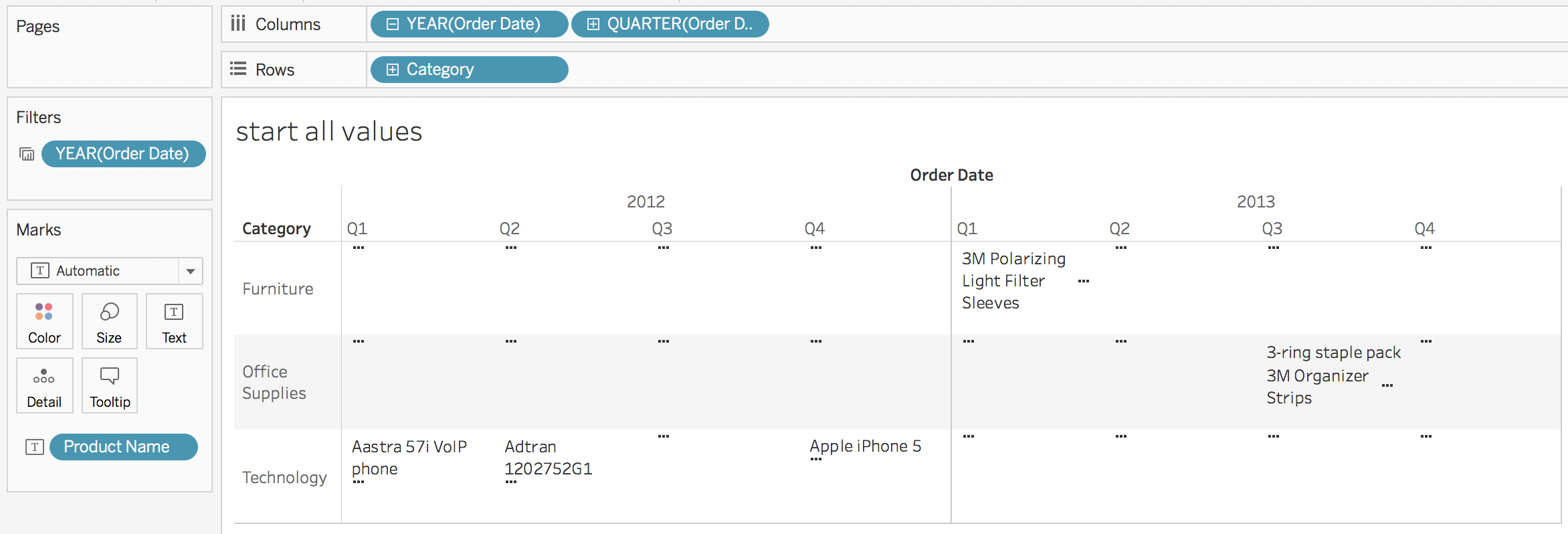
There’s a whole bunch of ellipses (…) where there’s too much data to display. The only options Tableau gives us in this case are to:

  • Change the order of the text by sorting the Product Name dimension.
  • Manually change the size of each pane by resizing the headers.
  • Use the Fit options to dynamically Fit Width, Fit Height, or Entire View.

The manual sizing is problematic because it won’t dynamically adjust to the number of marks, and in the case of views with lots of marks like this one it takes a lot of effort to figure out what size will get all the marks, never mind that the list of values is really hard to read:

And while the Fit options are great at ensuring a view with only a few marks takes up the available space when there are many marks it ends up either not displaying values or creating overlapping values depending on the settings.

Controlling X + Y

In this view the mark layout–either no pills or only discrete (blue) pills on Rows and Columns– is generating a pane for each distinct combination of header values and then Tableau’s mark stacking algorithm is laying out the text. So at this point we’re stuck and can’t do anything about what Tableau is up to. This is where we need to keep in mind one of the master Tableau concepts: everything is a scatterplot. If Tableau won’t place the marks where we want them then we can generate our own X + Y coordinates whether by adding data or creating our own calculations. This is the approach taken by the tile maps introduced to Tableau by Brittany Fong or or as a model of the solar system that I made awhile back: . More recently Ken Flerlage did a great introduction on his Beyond Show Me series of blog posts.

Therefore “all” we need to do is figure out where to place the marks. More on that in a moment, there are two more details I want to go into:

Green Panes vs. Blue Panes: Pane Sizing

Tableau’s logic around what generates a pane vs. marks in a pane is a little complicated so I’m going to keep this focused on three key elements, here are the first two:

  1. All panes created by a given combination of pills are the same size.
  2. (corollary to #1) If we resize one header or axis then all the other panes for that header or axis will resize as well. Tableau does this because it’s easier to visually parse (read) a view that has consistent sizing of elements.

Here’s a view with COUNTD(Product Names) on Text & Color with just discrete (blue) pills on Rows and Columns:

Somehow we need to fit 509 Product Names into the pane for Q4 2015/Office Supplies. If I resize Office Supplies to be taller then both Furniture & Technology change as well:

The same goes if I’ve got a continuous axis to place X/Y coordinates on. In this view I’ve simply put MIN(0) and MIN(1) on Columns & MIN(0) Rows and we can see a set of axes:

If I resize MIN(1) on Columns then to make it wider then all of the panes for MIN(0) and MIN(1) on Columns are resized.

So we can’t really dynamically resize panes to fit the data, all we can do is fit more or less into a pane. Therefore the desired solution can’t involve resizing panes, instead we will need to be generating more or fewer panes, and that leads to the next point around panes.

Green Panes vs. Blue Panes: Number of Panes

The third key element around green panes and blue panes is this:

  1. a) Continuous pills generate an axis for every discrete pill header. b) Discrete pills generate a header for every value of the pill.

We can see a) in action in the continuous views above, with MIN(0) and MIN(1) on Columns we get two axes for each quarter/year combination. So to add more axes we’d need to add more continuous pills but we can’t dynamically add them, and the number of axes ultimately depends on the discrete pills anyway so discrete is the way to go.

We can see b) in the discrete views above, there’s a header for each quarter in each year. Where this gets a little more interesting (and more useful in our case) is when the data is sparse, as in this case where the Avery products are not sold in every customer Segment:

Avery 5 is only sold in one segment so there is only a single header for Consumer, whereas Avery 494 is sold in all three segments so there’s a header for each.

So how this comes together is that in reating X/Y coordinates for positioning the text in our desired view we’re going to use discrete headers that can give us just enough headers (and no more) for the task, here’s a pic of the desired view with those headers:

Packing the Marks: the Algorithm

I experimented with some different layouts and looked at the following factors:

  • In each pane there’s a list of 0 or more values (marks).
  • At least in English when we’re reading lists we tend to make them top to bottom and when more is needed we add another column to the right.
  • There’s a balance in readability between too many columns vs. too tall columns. When there are many columns already then adding more columns for the list makes the view harder to read; in other words, a “tall” view with fewer columns is easier to read than a “wide” view.
  • When the panes in a row or panes in a column have different numbers of marks it’s important to efficiently stack the marks: too much white space can make the view harder to read.
  • A stacking layout that is closer to a differently-sized squares is easier to read than one that ends up with differently-sized rectangles.

The algorithm I came up with is a variation on the panel chart layout I used in Waffle Charts and Unit Charts on Maps that uses table calculations. The algorithm does the following:

  • Calculates the index for each mark in a pane using INDEX() and the number of marks in a pane using SIZE(). These calculations are used in the following calculations.
  • Counts the number of mark columns needed for each pane where there’s a Max # of Mark Columns. parameter to set a “no more than” value to prevent views from getting too wide. Then a nested calculation counts the maximum number of mark columns in each column.
  • Once we have the number of mark columns then the algorithm computes the number of mark rows for each pane, and then gets the maximum number of mark rows for each row.
  • Finally the mark row position and mark column position can be computed based on the index for each mark in the pane and the available number of rows and columns.

I numbered the calculations so they can be each brought into a workout view in order with their compute using set and validated before moving to the next calc. Calcs 1 & 2 require a compute using on the dimension to be used on Text and Calcs 4 & 6 have nested compute usings, see the comments on the calcs for details.

Here’s the workout view:

One complication is that the date dimensions are on Detail with custom dates with the ATTR() aggregation on Rows. This is a method to prevent unwanted data densification.

Once the workout view is built and validated then it’s possible to duplicate the view and rearrange pills, here’s that view:

There’s still a bit of manual resizing required, in this case it’s just to have enough size in each of the panes created by the column and row position table calculations to display the text. Once that is done those headers can be hidden for the final view:

We’re not limited to a text display, for example here’s a highlight table that only took a couple more clicks:


Conclusion

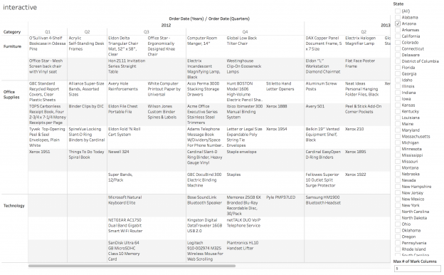
Here’s a view to play with where you can adjust the Max # of Columns parameter and the number of states (which is a proxy for how many products are displayed). Click the image to open the text wrapping in pane view on Tableau Public:
The key concept to keep in mind is that when Tableau won’t plot marks where we want we can add to the data source to get the necessary X&Y coordinates via joins, blends, and/or writing calculations. Since Tableau was designed as a tool to support interactive visual analytics tasks like making giant text tables with the desired text wrapping can take more effort than we might like, however given Tableau’s flexibility we can get the job done.
Waffle Charts and Unit Charts on Maps

One of the people I really wanted to meet at #data17 was Sarah Battersby, if you haven’t seen her blogs on mapping you’re missing out. It turns out she wanted to meet me, too!

So Sarah does really awesome stuff (can you tell I’m a fanboy yet??) and yesterday she posted about doing spiral jittering on maps:

That inspired me to dig out an old post where I’d done a waffle chart or unit chart jittering technique on a time series:

And adapt that to a map, like this one that makes me think of bunches of grapes:

Why would we need to do this?

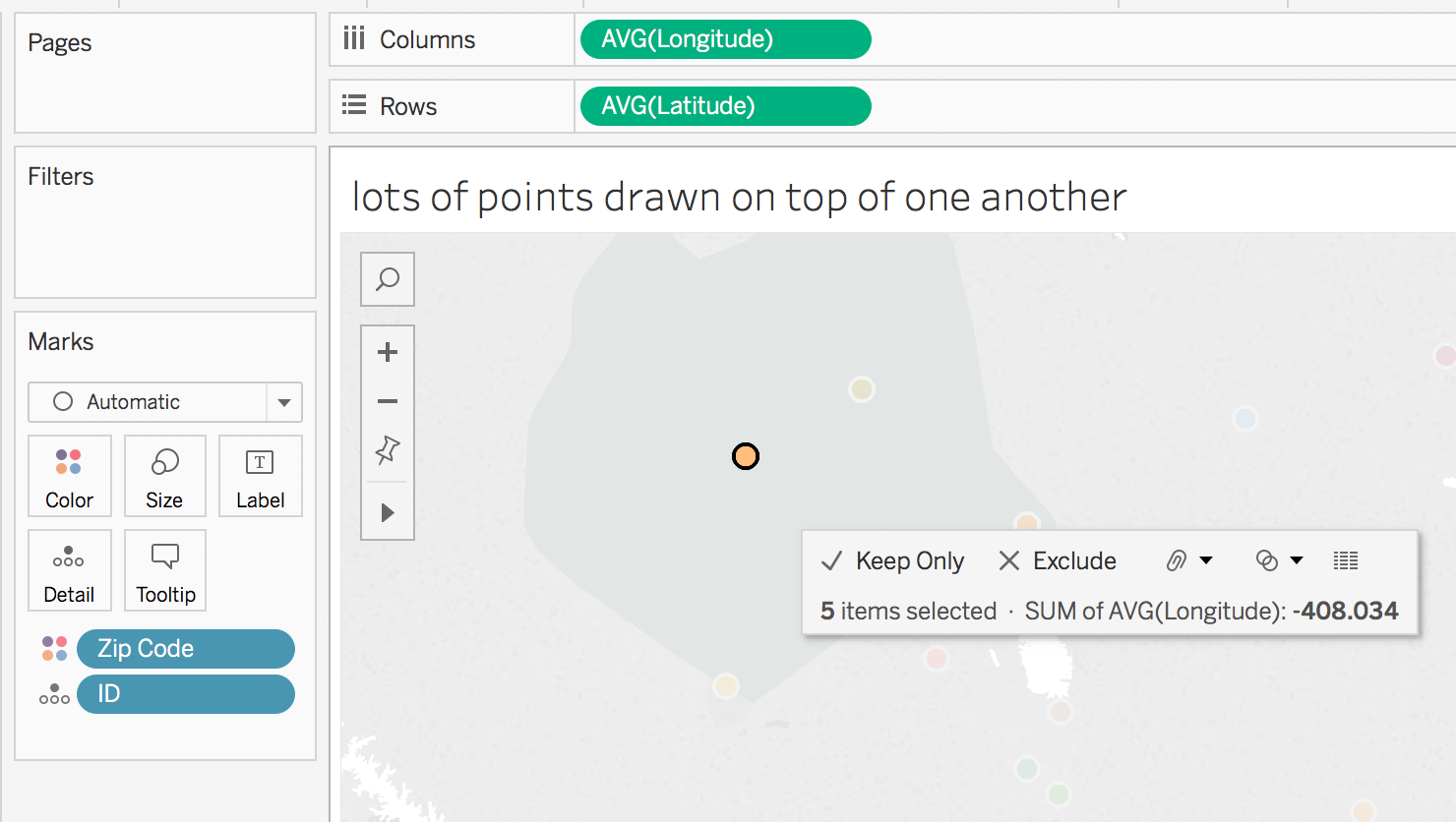
I’m not going to go into all the details, you can go read Sarah’s fantastic Jittering post instead for an overview. Basically there are times when we have more than one “thing” for one or more point(s) on a map and we want to show them that way. For example in the map below there are 5 IDs for the selected zip code that are all plotted on top of one another. Through using jittering we can show a mark for each ID like in the jittered map above where that one visible circle is replaced by five circles.

There is nothing new under the sun

Back in 2013 Stephen Few proposed the idea of bricks on maps as a way of encoding a value, the technique I’m using here could be used to get the same result. The key difference is that instead of using the unit or waffle chart to encode the single value we’re using the unit chart to encode multiple values. Andy Cotgreave also had a nice post on some of the issues with this kind of chart.

How do we put a waffle chart on a map?

First of all we need a data source that has latitudes & longitudes that we can do calculations on. If you don’t there are a variety of ways to get one. After that we need to get mathy. Here’s my workout view:

All of the table calculations have a compute using on ID, the idea is that the compute using is set to the dimension(s) that are making the extra marks and then the dimension(s) left for partitioning (Zip Code in this case) are the ones that are creating the initial map positions.

I’ll briefly walk through each calculation.

Index uses Tableau’s INDEX() formula and uniquely identifies each mark.

Column Count gets us a count of columns that is based on forming the smallest possible square that will contain all the marks, here’s the formula:

//this formula will try to draw a square, if you want something else then just put in a fixed aggregate number like MIN(3)
IF INT(SQRT(SIZE())) == SQRT(SIZE()) THEN
 SQRT(SIZE())
ELSE
 INT(SQRT(SIZE()))+1
END
This would be a lot simpler if Tableau supported the CEILING() function for table calculations, because then it would be CEILING(SQRT(SIZE())). Vote up https://community.tableau.com/ideas/6239 if you’d like that too.

Column Offset then computes the number of positions of lateral (latitude) offset for each mark from the center of the unit chart. I’ve done some different experiments on where to position the unit chart and for me the most natural is to have the center of the unit chart be the centroid of the point.

//this gets the column position in the row
IF [Index] % [Column Count] = 0 THEN
 [Column Count]
ELSE
 [Index] % [Column Count]
END
//subtract the position of the midline to get the offset
 - ([Column Count] + 1)/2

Row Count then gets the number of rows in the unit chart, and would again benefit from a CEILING() function for table calcs (hint hint).

IF INT(SIZE()/[Column Count]) = SIZE()/[Column Count] THEN
 SIZE()/[Column Count]
ELSE
 INT(SIZE()/[Column Count]) + 1
END

Row Offset computes the number of positions of vertical (longitude) offset for each mark from the center of the unit chart:

//row position in column
IF INT([Index]/[Column Count]) = [Index]/[Column Count] THEN
 [Index]/[Column Count]
ELSE
 INT([Index]/[Column Count]) + 1
END
//subtract the midline of the row to get the offset
- ([Row Count] + 1)/2

Jitter – Waffle – Latitude then gets the latitude for the point and subtracts the row offset multiplied by a waffle jitter parameter that lets us deal with the zoom level to offset by just the right amount of latitude. This field has the Latitude geographic role assigned.

TOTAL(AVG([Latitude])) - [Row Offset] * [waffle jitter]

Jitter – Waffle – Longitude does the same for the longitude.

TOTAL(AVG([Longitude])) + [Column Offset] * [waffle jitter]

Note that I’ve only tested this so far with US latitude & longitudes, these calcs might need to be slightly different if you are east of 0 longitude or south of the equator.

Building the View

With all the calcs created in the workout sheet and verified, then we can duplicate that sheet and start dragging & dropping pills to build a view. In this case I’ve created a dual axis on to show that the centers of the unit chart are on the centroids of the zip codes (the black crosses) and at this zoom level a waffle jitter value of 0.02 works well:

For this view I’ve made the waffle jitter slightly smaller to 0.015 degrees and added white borders to the marks:

Why Stop Here?

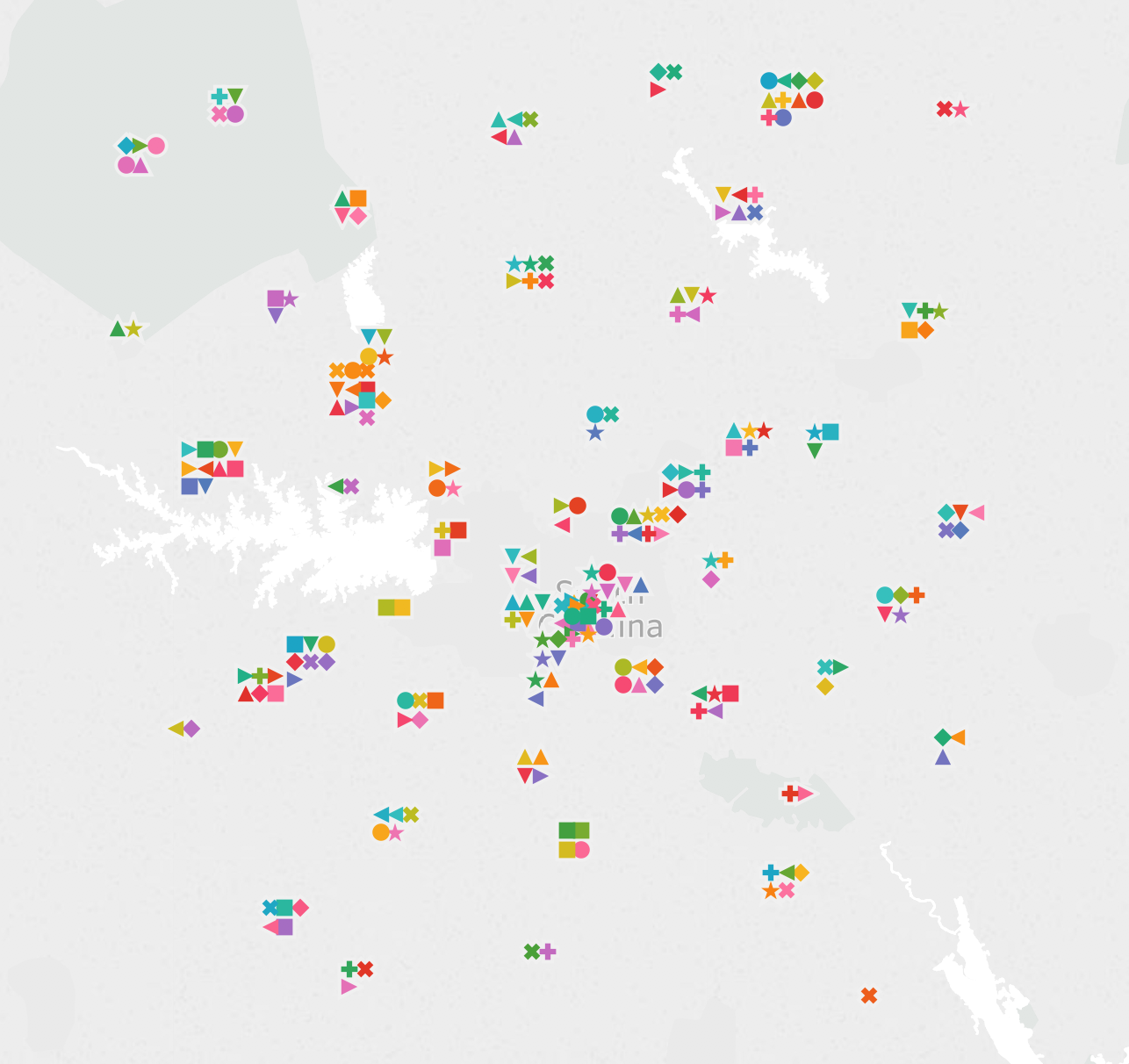
We don’t have to use just circle marks, in this view I’ve used shape marks and different colors for each shape just to show how much information we could place on a single view.

And in Tableau v10.5 we could even do something like only show the unit chart on a map if there weren’t too many marks nearby (by using a binning or hex bin function in an LOD expression) and use the new Viz in Tooltip feature to get the detail.

Conclusion

Thanks to Alan Eldridge for the original jittering post and Sarah for adding more jittering options and inspiring this post! Here’s the unit or waffle chart jitter on maps workbook on Tableau Public.


When 576 = 567 = 528 = 456: Counting Marks

Tableau’s data densification is like…nothing else I’ve ever used. It’s a feature that is totally brilliant when it “just works” like automatically building out a running sum on sparse data and mind-taxingly complicated when a data blend’s results go haywire because densification was accidentally triggered.

What I’ve historically taught users is to always ALWAYS look at the marks count in the status bar as a first way to detect when data densification occurs. Here’s Superstore Sales data with MONTH(Order Date) on Columns, Region and State on Rows, there are 499 marks and we can see that the data is sparse by the class that are missing Abcs:

Screen Shot 2016-08-16 at 11.52.15 PM

If I add SUM(Sales) to the Level of Detail Shelf and set it to a Running Total Quick Table Calculation with the default Compute Using of Table (Across) so it’s addressing on Order Date then I see 576 marks and all the Abcs are filled in, this is Tableau’s data densification at work:

Screen Shot 2016-08-16 at 11.55.19 PM

However, here are three additional views all still using the same pill layout and Quick Table Calculations  showing three different marks counts (567, 528, and 456):

Screen Shot 2016-08-16 at 11.59.11 PMScreen Shot 2016-08-17 at 12.00.55 AM

The marks count is changing based on a variety of factors, the different quick table calculations used (running total, difference, and percent difference) are a part of it but the underlying behavior depends on whether a mark is densified or not, the pill arrangement, and whether or not a densified mark has been assigned a value (including Null) or not. Prior to Tableau version 9.0 these all would have been counted in the marks count and the views would show 576 marks for each, Tableau v9.0 changed the behavior to only count the “visible” marks.

I’ll walk through the above there examples. In this one the Running Total has been moved from the Level of Detail to the Rows Shelf and there are 567 marks.

Screen Shot 2016-08-16 at 11.59.11 PM

The reason why is that even though those combinations of Region, State, and Month have been densified for states like Iowa that don’t have any sales in the first month(s) of the year (more on how I know that below) those densified marks don’t have any assigned value (even Null) so they are not counted in the marks count nor are they counted in the Special Values indicator in the lower right.

In this view using the Difference calculation there are 528 marks and the Special Values indicator shows 48 nulls (528+48 = 576). In this case the Difference calculation is using the LOOKUP() function that is returning Null for the densified values.

Screen Shot 2016-08-16 at 11.59.11 PM

Finally in this view using the % Difference calculation there are 456 marks and the Special Values indicator shows 120 nulls (456+120 = 576). In this case the % difference calculation is spitting out extra nulls due to divide by 0 results.

Screen Shot 2016-08-16 at 11.59.11 PM

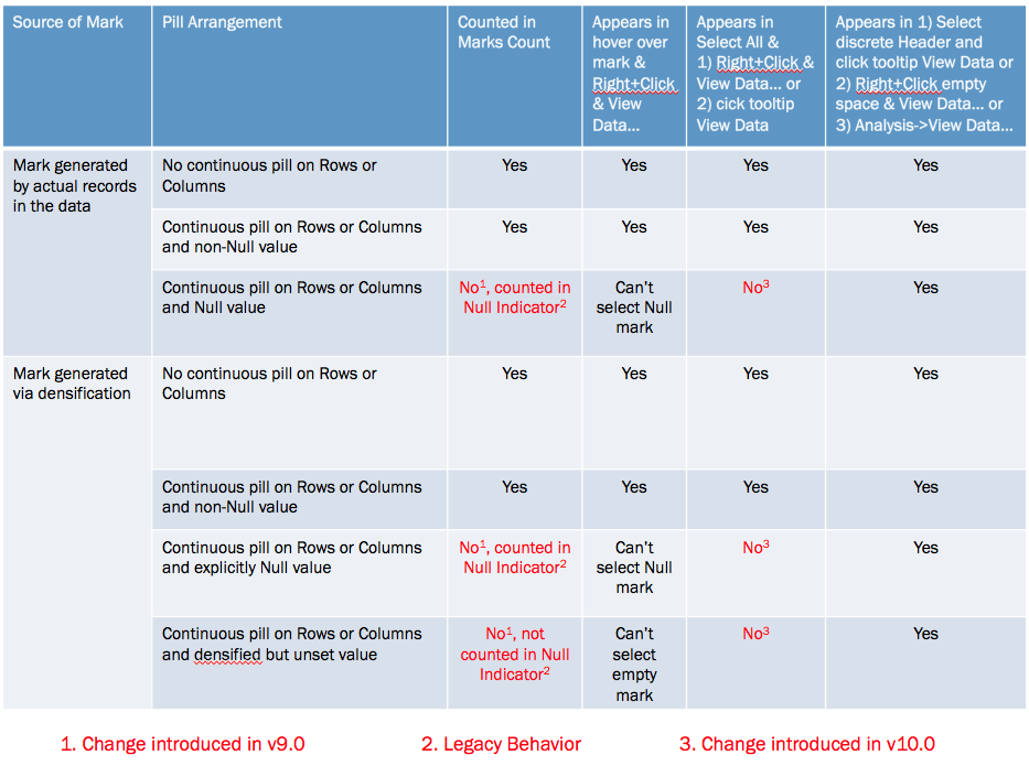
The difference is due to a change made in Tableau v9.0 where the marks count now only counts “visible” marks (Tableau’s term), where the definition of a “visible” mark is complicated, they are the “Yes” answers in the table below:

Screen Shot 2016-08-17 at 12.09.17 AM

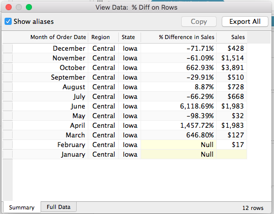
Now one of the ways I’ve been used to checking for densification is selecting all the marks (either by Right+Clicking and choosing Select All or pressing Ctrl/Cmd+A) and then hovering over a mark and Right+Clicking and choosing View Data… or waiting for the tooltip to come up and using View Data. For example here’s the select all View Data in v9.0 for the % Difference on Rows view, the yellow cells indicate where data was densified and there are 576 rows:

Screen Shot 2016-08-17 at 12.12.24 AM

However, that doesn’t work anymore in Tableau v10.0, there was change made to the Select All functionality such that Select All only gets the “visible” marks, here’s that same view data in v10 and there are only 456 rows:

Screen Shot 2016-08-17 at 12.12.58 AM

So Select All doesn’t work the way it used to, and the marks count can change in “interesting ways” (and we haven’t gone into what things like formatting Special Values can do), so what can we do to spot densification? There are three workarounds for this, all documented in the right-most column of the table above:

  1. Select a discrete header or a range of headers, wait for the tooltip to come up, and click on the View Data icon.
  2. Right-click in the view (but not on a mark) and choose View Data…
  3. Use the Analyis->View Data… menu option.

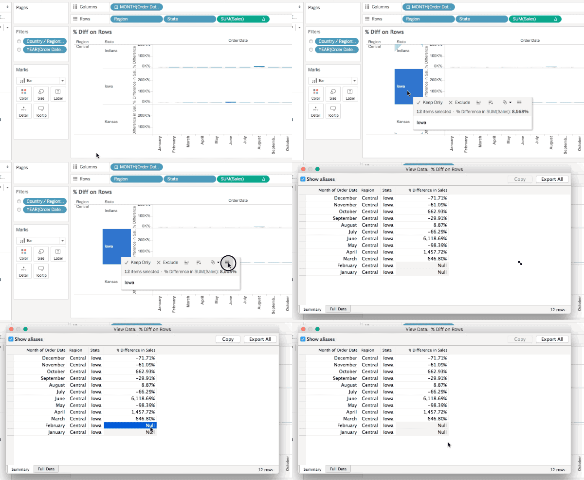
All of these will show the densified values, here’s an animated GIF of selecting Iowa selected in the Difference on Rows view where we can see the  two Null values:

2016-08-17 00_21_03

However only one of those is actually densified, to tell that exactly we need to add a field that actually has data. In this case I’ve added SUM(Sales) to the Level of Detail Shelf and the View Data for Iowa now shows that it’s really only January that is densified, since there’s nothing at all in the January SUM(Sales) cell:

Screen Shot 2016-08-17 at 12.27.28 AM

Conclusion

The marks count is not a reliable indicator of the volume of densification and we need to resort to various selection mechanisms and the View Data dialog to more specifically identify how much has been densified. I’m not a fan of these changes: what I’d really like Tableau to do is to add a count of densified values to the status bar and details on what was densified to the default caption and the Worksheet->Describe Sheet… Until that time, though, hopefully this post will help you keep track of what Tableau is doing!

Here’s a link to the marks count workbook in v8.3 format (so you can open it up for yourself and see the differences in different versions).

Sorting a Dimension by Two Values At Once

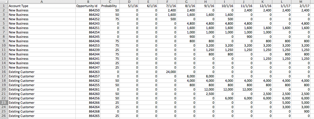
I recently got a question via email about how to sort a view by two different criteria at the same time. Here’s an Excel table of opportunities where for each month and Opportunity ID there’s a forecast of size of opportunity:

Screen Shot 2016-06-30 at 2.12.45 PM

The goal here is to sort the opportunities within each account type by the nearest (by month) and biggest opportunities (by Forecast size) first, so it looks more like this in Tableau:

Screen Shot 2016-06-30 at 2.13.38 PM

Now with that data in Excel arranged in a tabular form I can sort on December, then November, then October, and so on, and get the desired sort:

Screen Shot 2016-06-30 at 2.14.29 PM

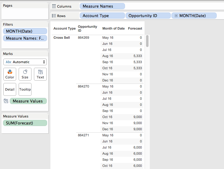
But in Tableau I can’t do that, if I try to work with the data in that “wide” format with a column for each month it just won’t work. If I use Tableau’s pivot feature to make the data “tall” with a record for each Opportunity ID and Month then I still run into problems. I want to sort the opportunities by each month and by Forecast but when I try to sort the Opportunity ID dimension I can’t get it to work, it only sorts by a single month’s values, so in the view below Opportunity ID 864280 should be the first new one for August since:

Screen Shot 2016-06-30 at 2.15.31 PM

The Excel way isn’t good because each month I have to manually re-sort the data. And in Tableau it just seems impossible to get the right sort because it looks like we need to sort in two different directions at once (get the earliest non-zero month for each opportunity, and then sort up and down the opportunities in each account type), and Tableau only lets us sort on one thing at a time. However, it is possible – read on for how to get this kind of sort in Tableau and maybe learn a few math tricks!

Part of how this kind of problem can be more challenging is the way the problem (and data) is initially presented to us. When we see the data in the crosstab form in Tableau the *appearance* is that we need to sort in two different directions. In fact, we really only need to sort in one direction based on the forecast value in the first month for each opportunity, so in the view below we’d want Opportunity ID 864271 to be the first one sorted because it’s from July 2016.

Screen Shot 2016-06-30 at 2.16.45 PM

Each opportunity row in the view needs to be sorted within the account type by the first (earliest) month where there is a non-zero forecast and then by the value of Forecast in descending order for that month.

The key to sorting headers and panes in Tableau is that it’s done using the discrete (blue) pills on Rows or Columns from left to right. So the left-most discrete (blue) pill headers are sorted, then the 2nd discrete pill’s headers are sorted, and so on. For discrete dimensions from a primary source we can sort by a measure, use the default alphanumeric sort, or a manually, otherwise any discrete pills are by default alphanumerically sorted or manually sorted.

Therefore in this case I knew I needed to either return a measure that could sort some dimension (like the Opportunity ID) or return a discrete dimension value that with the default alphanumerical sort would work right. Note that filtering wouldn’t work here because the goal is to show a sorted crosstab.

The next part of working out the solution is how to structure this value for sorting. I’ve done some multi-level sorting in the past where I needed a nested sort of single dimension by two different criteria, and a common construct is a number of the form X.Y where the integer portion X is from one criteria and the decimal portion N is from the other criteria. So with the default alphanumerical sort 1.2 comes before 1.3 comes before 2.1 etc.

So for the integer part of the sort I need to convert the date for each opportunity into a number where the Forecast is greater than 0. The Date Number (temp) calc has the formula:

IF [Forecast] > 0 THEN
    INT([Date])
END

Screen Shot 2016-06-30 at 2.17.34 PM

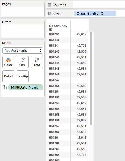
This convers the date into an integer, in this case the number of days since 1/1/1900. To get the first (earliest) month for each opportunity then all I need to do is aggregate it with MIN() at the level of Opportunity ID:

Screen Shot 2016-06-30 at 2.18.01 PM

Ultimately, this is is what we’re going to do to get that pill sort of Opportunity ID’s in the final view.

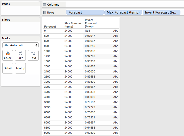
For the decimal part of the sort I needed a number where the smallest numbers reflected the largest values, and it needed a value between 0 and 0.999999 (it can’t be a whole value of 1 because that would affect the integer sort). A way to turn a set of positive numbers into decimal numbers between 0 and 1 is to do X/(max X). In this case X is the Forecast, so to get the max X in the data I used the Level of Detail Expression, here’s the Max Forecast (temp) formula:

{FIXED : MAX([Forecast])}

Screen Shot 2016-06-30 at 2.18.35 PM

Now if I do [Forecast]/MAX([Forecast]) that’s going to return a number between 0 and 1 that preserves the original ordering of values, i.e. bigger values of Forecast are closer to 1. So to invert that I used use 1 – X/(max X). So if (max X) is 10 and X is 9, then the result of (1 – 9/10) is 0.1, while if X is 2 then the result of (1- 2/10) is 0.8, a bigger number.

We avoid results of 1 that could affect the sort by skipping values of where the Forecast is 0, here’s the Invert Forecast (temp) formula:

IF [Forecast] > 0 THEN
    1-[Forecast]/[LOD Max Forecast Value]
END

Screen Shot 2016-06-30 at 2.19.19 PM

I could have avoided the LOD expression for the max value by just setting a gigantically huge number, however past experience with foreign currencies has shown me that whatever huge number I can imagine is likely to be smaller than reality so I chose to make sure that the value is coming from the data

With all the values worked out I could now put everything together into a single calculation, this is the Sort calc that returns record-level values:

IF [Forecast] > 0 THEN
    INT([Date])
    + (1-[Forecast]/{FIXED : MAX([Forecast])})
//Forecast is 0, return a really big number that will be put at the end of the sort
ELSE
    999999
END

Screen Shot 2016-06-30 at 2.20.09 PM

This calc returns the numbers as record level values.

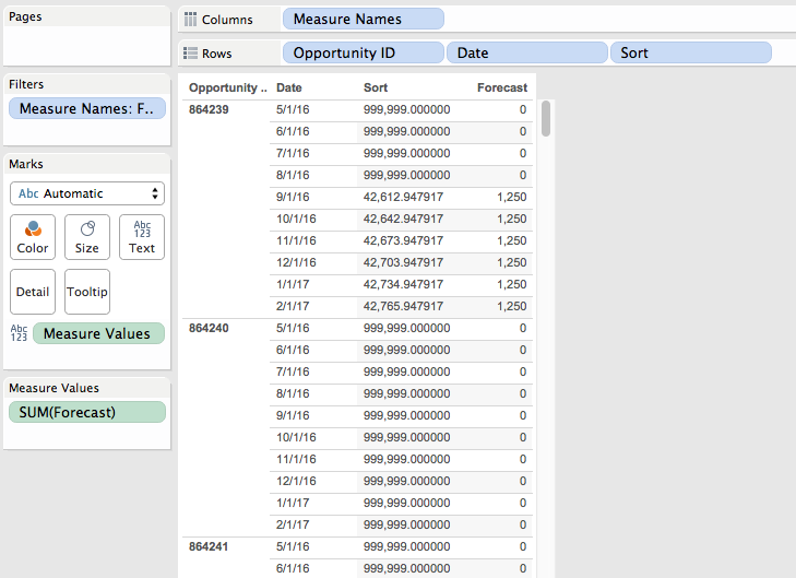
To show how the sort works out I set up this view where the Sort calc is used as the leftmost discrete dimension to show what gets sorted first, with the bar chart we can quickly visually verify that the dates are sorted with earliest months first and then by the Forecast within each month:

Screen Shot 2016-06-30 at 2.20.41 PM

Note that there’s a different value for each Opportunity ID/month combination, when what we really want is that single minimum value for each Opportunity ID/month. So we need to aggregate the Sort measure with MIN() at the level of detail of Opportunity ID, and we can do just that using a pill sort on the Opportunity ID dimension:

Screen Shot 2016-06-30 at 2.21.14 PM

Now we can arrange pills to build the original crosstab view and have the desired sort:

Screen Shot 2016-06-30 at 2.13.38 PM

And as the data updates the sort will automatically work, in this case I’ve added January 2017 to the data:

Screen Shot 2016-06-30 at 2.22.37 PM

Conclusion

The following bits of Tableau knowledge were necessary to get the desired results:

  • How Tableau sorts views using discrete pills.
  • How Tableau’s pill sorts work.
  • A tiny bit of Level of Detail Expression building.

And then the following math tricks were used:

  • Combining two different numbers into one using an integer number for one value and a decimal number for the second value.
  • Making positive numbers into a range of 0-1 using X/(max X). A different formula would be needed if there were negative numbers and/or the desired range was different.
  • Inverting ranges to make big numbers small and small numbers big using 1 – X/(max X)

FYI if LOD expressions are not available in your particular data source then you could use a table calculation, a data blend, or just manually enter your equivalent of the Max Forecast value. I set up a table calculation version as well in the Sorting by Two Values Tableau Public workbook.

Show Me *All* The Numbers: Displaying Every Record for Too Tall Data

Here’s a sample data set with 4 records:

When we bring that data set into Tableau and build a text table, though, we only see 3 rows:

If we want to show all 4 underlying records as 4 rows in the Tableau text table we have to jump through a couple of hoops, the rest of this post describes why Tableau behaves that way and how to fix it.

The Data is Too Tall

There are all sorts of resources about working with data that is “too wide”, for example the old Preparing Excel Files for Analysis KB article, the new Pivot feature introduced in Tableau v9.0, or this post on Tiny Habits from Emily Kund with commentary from yours truly. Too wide data has too many columns for the kind of analysis that we want to use. There aren’t so many resources on “too tall” data, of which this is an excellent example.

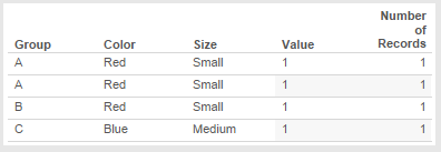
To explain what “too tall” data is, let’s first look at the data:

What is the grain of this data? In other words, what combination of field(s) makes a unique record in the data?  We might be tempted to say Group, Color, and Size, but for Tableau there is no difference between the first two records:

Effectively the data has no unique grain. Yes, there’s a difference in position between these two records but that is not detectable by Tableau because record order (position) is not something stored in each record. This highlights something I talk about in my training classes: the difference in mental models between Tableau and WYSIWYG tools like Excel. Tableau approaches data as a database does, and the default behavior in databases is that record order doesn’t matter. The reason databases abstract record order away is to get higher performance.

So when we bring this data into Tableau and create a view Tableau’s default behavior is to aggregate the data to the level of the dimensions in the view (i.e. on all Shelves and the Marks Card except for Filters). Here’s what happens we bring all the fields in this data set into the view as dimensions:

There aren’t enough dimensions to separate out the two A/Red/Small records. This explains what I wrote earlier about the data lacking enough dimensionality. What we really need is another column (field) to identify the records. So we now have a simple definition:

  • “too tall” data has too few columns to effectively perform the analyses we want
  • “too wide” data has too many columns to do effectively perform the analysis we want

The rest of this post describes three ways to show all the records: Show Underlying data, editing the source, and constructing a specific Tableau view.

Do You Need to Show the Data in a View?

If you don’t need to show the data in a Tableau view users can still view the underlying data in both Tableau Desktop and from Tableau Server & Online. Here’s the underlying data in Tableau Desktop:
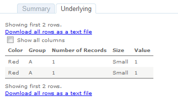
And on Tableau Server:

So some user education might be all you need to show all the records. If the data is too tall and you do have to show a view with all the records then you can alter the source data or set it up in Tableau.

Do You Control the SpiceSource?

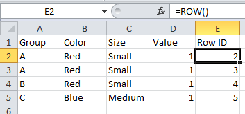
If you have control over the source data then many sources have features to add a unique record identifier that would add that necessary column to make the data not too tall, not too wide, but just right. For example Excel has the ROW() function:


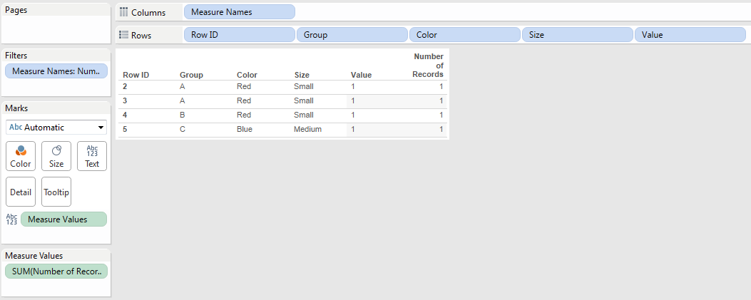
Creating a view with this that shows every record is trivial, we just need to add Row ID as a dimension:

If you’re not using Excel then you’ll need to look for a function that adds a row ID, record ID, etc. Part of why this is a rare problem is that most relational data tables are set up with unique keys (indexes) that give us those unique values to draw tables. Where I typically see too tall data coming from is from hand-entered data sources and ancient systems.

When you don’t have that option and you’re stuck with too tall data we can still get a view showing every record in Tableau.

Building a Tableau View Showing Every Record for Too Tall Data

There are three main steps to building a view to show every record:

  1. Turning off aggregation so Tableau will return every record from the data source.
  2. Creating a table calculation to increment over each record and provide a unique identifier.
  3. Using that table calculation as a discrete pill to sort the view.

Here’s how using the above data source:

  1. Turn off Analysis->Aggregate Measures:

    The view now looks like this:

    The reason why there’s a lot of white space is that Tableau is now returning multiple records (the two 1’s) for A/Red/Small and has turned on Mark Stacking by default. This is not a problem, we’ll be rearranging the view later on to get rid of Mark Stacking.
  2. Create a Rank calculated field with the following formula:
    RANK_UNIQUE(MIN([Number of Records]))

    I use RANK_UNIQUE() here instead of INDEX() because rank only counts non-Null values and should there be any unwanted densification those ranks will return Null, whereas INDEX() would return values that would throw off the desired ordering.

  3. Drag the Rank field to the Level of Detail Shelf and set the Compute Using to an Advanced… Compute Using where all the dimensions are used for addressing in the order that you want the records to appear:

    Something I’ll typically do at this point to validate is to add the table calc (Rank) to the text Shelf or Measure Values (here I have it on text):
    And we can see that the Rank is accurate.
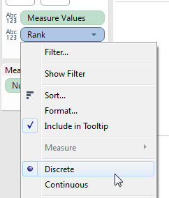
  4. Turn Rank into a discrete (blue) pill:
  5. Drag Rank to the Rows Shelf to the left of all the dimensions. With the unique identifier for each record (mark) the Mark Stacking goes away:
  6. As the last step turn off Show Headers for the Rank pill:

    The view now shows each individual record:

Conclusion

Tableau is designed to help us dive & swoop through thousands/millions/billions of rows of data to discover insights so Tableau’s default behavior is to aggregate the data. Tack on Tableau’s mental model of treating data as a database does and a task like showing every record can be more complicated when the data source isn’t aware of more modern database concepts and lacks the necessary dimensions to uniquely identify each record. A feature request for row numbering has been created to make this easier, vote it up if this is something that interests you!

Here’s a link to the too tall workbook on Tableau Public.