In all the hype about big data, we have to acknowledge that some of us have “wee” data. Not every organization has a fully-built out Information Systems department or Business Intelligence team with access to petabytes of data and the latest tools like Hadoop and Alteryx. Some of us are still running on legacy hardware and software, have tiny budgets, part-time staff, and thousands or tens of thousands of records that we want to analyze vs. billions.
My day job is in the latter camp. For all that US healthcare includes the latest treatments and technology, healthcare IT has historically been behind the times. My desktop is running Windows XP SP3, Office 2007 is our productivity tool, Microsoft Access is our most commonly used database, and Tableau is our go-to choice for data visualization (so there’s at least one area where we’re we’ve got current technology).
Every couple-few months I get a question about Microsoft Access and Tableau, I thought I’d take a few minutes to combine my answers into one post, so read on for what I know about integrating Access and Tableau.
This post was updated on 24 July 2015 to include additional details on applying the custom formatting calculation to aggregates.
Here’s a quick lunchtime post on working with durations in Tableau. By duration, I mean having a result that is showing the number of seconds, minutes, hours, and/or days in the form of dd:hh:mm:ss. This isn’t quite a built-in option, there are a several ways to go about this:
Use any duration formatting that is supported in your data source, for example by pre-computing values or using a RAWSQL function.
Do a bunch of calculations and string manipulations to get the date to set up. I prefer to avoid these mainly because they can be over 1000x slower than numeric manipulations. If you want to see how to do this, there’s a good example on this Idea for Additional Date Time Number Formats. (If that idea is implemented and marked as Released, then you can ignore this post!)
If the duration is less than 24 hours (86400 seconds), then you can use Tableau’s built-in date formatting. I’ll show how to do this here.
Do some calculations and then use Tableau’s built-in number formatting. This is the brand-new solution and involves a bit of indirection.
Durations Guaranteed To Be Less Than 24 Hours: Tableau’s Date Formatting
If you know your duration is always going to be less than 24 hours (86400 seconds), , then you can take advantage of Tableau’s built-in date formatting. The first step is to get your duration in seconds, if it’s not already. For example, for looking at the duration between two dates you can use DATEDIFF(‘second’,[Start Time], [End Time]). Once you have that number of seconds, then you can use the following calculation
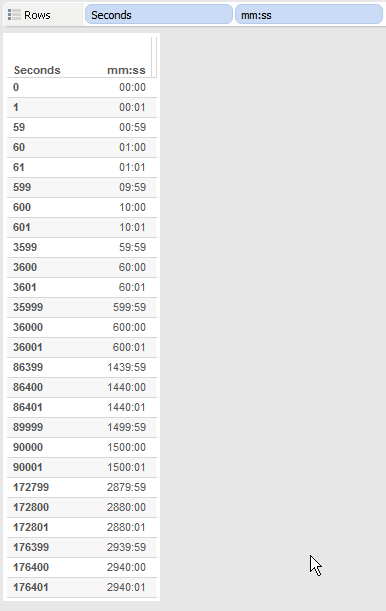
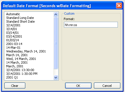
If the total time is less than 24 hours, then we can use the following calculation: DATETIME([Seconds]/86400). Then we can use Tableau’s date format to set the format as hh:nn:ss (in this case hh:mm:ss will also work):
Here’s a view…take a look at what happens at 86400 seconds and beyond:
Instead of showing 24 hours, the date formatting looks just at the hours, minutes, and seconds. As long as your duration is less than 86400 seconds, everything will be simple using this technique.
Any Duration: Using Arithmetic and Number Formatting
Though Tableau’s built-in formatting is not as powerful as Excel, we can still do quite a bit. Check out Robert Mundigl’s Custom Number Formats for a pretty exhaustive list of what can be done. (He’s also got a fantastic post on String Calculations that is worth checking out.)
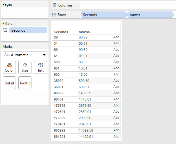
For example, we can set up a custom number format of 00:00, and that will perfectly format a number as a time…up to 59 seconds, that is:
However, this is a clue to the next step, which is that since we space out numbers by colons, all we need to do is get the right value into the right decimal place. So, for example, instead of 60 seconds (1 minute) being a value of 60, it has to have a value of 100 so the 00:00 formatting will make it 01:00. Here’s a formula that does just that for mm:ss values:
//replace [Seconds] with whatever field has the number of seconds in it
//and use a custom number format of 00:00:00:00
//(drop the first 0 to get rid of leading 0's for minutes)
IIF([Seconds] % 60 == 60,0,[Seconds] % 60)// seconds
+ INT([Seconds]/60) * 100 //minutes
In this formula, [Seconds] is a record-level field. In order for the calculation to work accurately in some situations (such as using it with Subtotals and Grand Totals) you’ll need to change [Seconds] to SUM([Seconds]) or some already-aggregated calculated field. –added 2014-12-22 per notes in the comments.
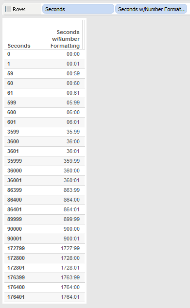
The formula uses the % (modulo) function to divide the number of seconds by 60 to get the remainder, the IIF statement is there to deal with what happens when the number of seconds is divisible by 60, the result of that is the number of seconds, then the number of minutes *100 is added to that. Here’s a view:
For hh:mm:ss the formula gets a little more complex. Just as the seconds had to be transformed to make 0-59 seconds, minutes have to do a similar transformation:
//replace [Seconds] with whatever field has the number of seconds in it
//and use a custom number format of 00:00:00 (drop the first 0 to get rid of leading 0's for hours)
IIF([Seconds] % 60 == 60,0,[Seconds] % 60)// seconds
+ IIF(INT([Seconds]/60) %60 == 60, 0, INT([Seconds]/60) %60) * 100 //minutes
+ INT([Seconds]/3600) * 10000 //hours
And for dd:hh:mm:ss there’s yet another transformation to convert hours to 0-23:
//replace [Seconds] with whatever field has the number of seconds in it
//and use a custom number format of 00:00:00:00 (drop the first 0 to get rid of leading 0's for days)
IIF([Seconds] % 60 == 60,0,[Seconds] % 60)// seconds
+ IIF(INT([Seconds]/60) %60 == 60, 0, INT([Seconds]/60) %60) * 100 //minutes
+ IIF(INT([Seconds]/3600) % 24 == 0, 0, INT([Seconds]/3600) % 24) * 10000 //hours
+ INT([Seconds]/86400) * 1000000 // days
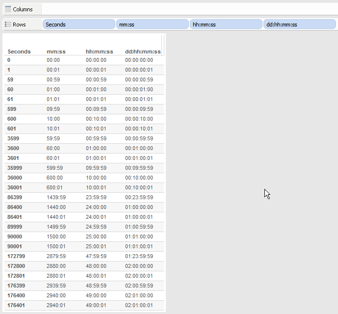
Here’s a view showing all three calculations:
A little dose of math, sprinkle some custom number formatting on it, and voila, there’s some usable duration formatting. If you wanted to keep going into weeks then there would need to be another level of calculation, to get into months and years I’d probably use a different approach because the intervals (month lengths and year lengths) aren’t fixed.
If this is useful to you, or you have an alternative technique, let me know in the comments below!
Addendum on Aggregation (July 2015)
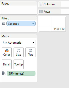
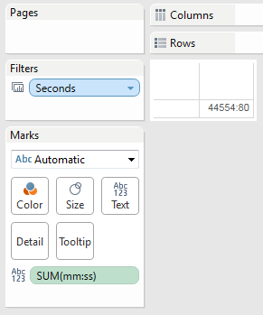
Some people people using this technique have run into problems as seen in the comments below and on the Tableau forums. For example, if we build a view like this and sum up all the values of Seconds with the duration calc applied (see the SUM() aggregation) the numbers don’t add up. In this view the total time in mm:ss should be 44558:00 but it’s showing up as 44554:80, a non-sensical amount:
Alternatively, if we keep Seconds in the view as a dimension but add a Grand Total, the Grand Total isn’t adding up either:
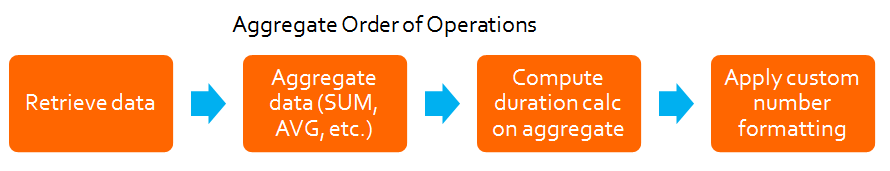
The issue is with regards to order of operations. When we build the views with the grand total or by summing the measure, there’s an aggregation happening and it’s not happening at the right time vis-a-vis the formatting. I put together a series of graphics to explain what is going on.
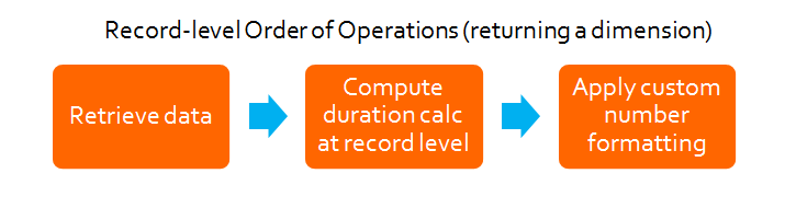
In the original post the duration calculations are performed for each record and the results are treturned from the view. So it looks like this:
So in this case here’s what’s going on under the hood:
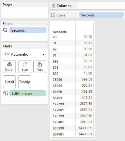
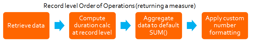
That’s not often used in practice, more often a view looks like this, where the mm:ss is being used as a measure and then when the original calculation is brought into the view we can see that Tableau is actually aggregating the duration calculation with the default aggregation of SUM():
However, that SUM() has no effect because the level of detail (the granularity) of the view is the same is the same as the data — in other words, the view is effectively displaying the raw data. So the order of operations is actually like this:
So even though these two views look exactly the same, under the hood they are using two different ways to get there. Where this causes problems is when we apply an aggregation that is across multiple records or in a grand total or subtotal. The duration calculation that was meant to be applied to the final result is being applied to every record and it’s that transmogrified amount that is getting summed:
The solution is pretty straightforward, we just need to do the aggregation *before* we apply the duration calculation. So instead of the [Seconds] of the original calculation we use Sum Seconds with the formula SUM([Seconds]), and the formula for mm:ss (agg) is:
//replace [Sum Seconds] with whatever field has the number of seconds in it
IIF([Sum Seconds] % 60 == 60,0,[Sum Seconds] % 60)// seconds
+ INT([Sum Seconds]/60) * 100 //minutes
So the order of operations is now:
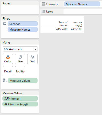
And here’s a view showing the inaccurate and now accurate aggregate calculations:
If you’re not off on some sunny beach somewhere (or even if you are), here are some (free!) opportunities coming up for you to sharpen your Tableau skills and get previews of material that will be in my book. I’ve got 3 presentations in the next month, two are in New England, the other is a webinar:
June 24th at the Boston Tableau User Group: Making Tableau More Predictable: Understanding the Multiple Levels of Granularity. This is a reschedule of the session I was going to give back in April, it’ll be a combination of presentation and hands-on practice on how to “think Tableau” so your calculated fields, top & conditional filters, table calcs, etc. are more likely to come out the way you expect. Alteryx is demoing their software, and Zach Leber is also presenting.
July 10th for a Think Data Thursday webinar: Setting up for Table Calculation Success. This will also review some of the granularity material, and go through how you can set up views and table calculations so that a) they work, and b) if they don’t work how to diagnose what is going on so you can get back to a working calc or be able to submit a really detailed support request.
July 22nd at the (inaugural) Maine Tableau User Group: Getting Good at Tableau. Hosted by Abilis Solutions in Portland, I’m helping to kick off the MaineTUG with a talk on how to set up your data and build your Tableau skills (including how to avoid getting distracted by all the gee-whiz features of the Tableau interface) and I’ll do some intro of Tableau 8.2. Grant Hogan of Abilis will be presenting, as well as someone from Tableau.
I’ll update this post as the links for registering appear, I hope to see you (virtually or in person) at one of these events! And if not then, I’ll be a the Tableau Conference in September.
There was a Tableau forums thread on At the Level awhile back where Matthew Lutton asked for an alternative explanation of this somewhat puzzling table calculation configuration option, and I’d promised I’d take a swing at it. Plus, I’ve been deep into book writing about shaping data for Tableau, and a taking a break to write about obscure table calc options sounds like fun! (Yes, I’m wired differently.)
Read on for a refresher on addressing and partitioning and my current understanding of uses of At the Level for ordinal table calculations such as INDEX() and SIZE(). Part 2 will cover LOOKUP(), and Part 3 will cover WINDOW_SUM(), RUNNING_SUM(), and R scripts. If you’re new to table calcs, read through at least the Beginning set of links in Want to Learn Table Calculations. Thanks to Alex Kerin, Richard Leeke, Dimitri Blyumin, Joe Mako, and Ross Bunker for their Tableau forum posts that have informed what you’re about to read.
A guest post by Noah Salvaterra, you can find him on the Tableau forum or on Twitter @noahsalvaterra.
I expect the header image may spark some discussion about visualization best practices; actually, I sort of hope it does. The data shown is from NOAA’s online database of significant earthquakes and is displayed by magnitude on a globe, so 4 dimensions packed into a 2 dimensional screen. While it was created in Tableau, it might be a long wait before something like this appears in the show-me menu.
For those who missed the header because they are reading this in an email, I’ve included an animated 3D version on the left, though to actually see it in 3D requires the use of ChromaDepth glasses (I discussed this technique in more detail in a prior blog post). Use of 3D glasses adds even more controversy because while we can get some understanding of depth from a 3D image, it isn’t perceived in an equal way to height and width. Data visualization best practices can help in choosing between several representations of the same dataset, choosing bar graphs over pies, for example, since bars will typically lead to a better understanding of the data. Best practices also instruct us to avoid distorted presentations such as 3D or exploding pies and 3D bar charts, since these are likely to lead to misunderstanding. I’m not exactly sure what best practices has to say about this spinning 3d anomaly, my guess is it would be frowned upon. I think there is something to be said for including a novel view of your data if it helps to engage with the topic, and even if this one does break some rules, it’s hard to look away. If you’d rather just see the earth spinning, without all the data overlaid, there is an earth only view at the end.
The images above may not be the best choice as general way to visualize this earthquake data. In fact, I’m the first to admit that it has some significant issues. Comparing earthquake magnitudes between 2 geographic areas would be tricky, plus half of the earth is hidden from view completely because it is on the back. Adding the ability to rotate the globe in various directions in a Tableau workbook helps a bit, but you’re left to rely on your memory to assemble the complete picture. If the magnitude of the quakes is the story you’re telling, you might be better served with a flat map maybe using circles to represent the magnitude of the quakes, such as the one shown below. I think this is a good presentation; it has some nice interactivity and as far as I know doesn’t break any major rules from a best practices standpoint. But it certainly isn’t perfect, nor is without distortion. Judging the relative size of circles isn’t something that will be perceived consistently, but the failure I had in mind isn’t one of perception, it is about the data being accurate at all. The map itself brings a tremendous amount of distortion to the picture, in location of all things.
In case you haven’t heard, the earth isn’t flat (I like to imagine someone’s head just exploded as they read that sentence). It is roughly spherical. Well, technically it is a bit more ellipsoidal, bulging out slightly along the equator, and more technically still this ellipsoid is irregularly dotted with mountains, oceans, freeways, trees, elephants and wal-marts (not meant to be a comprehensive list). Also, as the moon orbits, it causes a measurable effect not just on the tides, but it distorts the land a bit as well as it passes by. Furthermore, the thin surface we inhabit floats, lifting, sinking, circulating on top of a spinning liquid center. Earthquakes serve as a reminder of this fact. The truth can be overwhelming in its complexity; so we simplify. Though not the complete truth, a well-chosen model can be a valuable proxy when it doesn’t oversimplify. One way to understand the difference would be to analyze the scale of the errors introduced. The highest point on earth is Mt. Chimborazo in Ecuador at 6,384.4 km… you were thinking Everest? That is the highest above sea level, but the sea bulges as well, and Chimborazo is the furthest from the center getting a boost by being close to the equator. The closest point to the center of the earth is in the arctic ocean near the north pole and is about 6,353 km from center. If we use the mean radius of 6,371 we are doing pretty well (error is within .3%). A sphere seems like a reasonable compromise.
So the earth is spherical… but our map is rectangular. You don’t need to invest in differential geometry course to understand that there is something fishy going on there (though you might to prove it). In fact there is no way to map a spherical earth to a rectangle, or any flat surface without messing something up, the something being angle, size or distance; at least one will be distorted when the earth is presented on a flat surface (sometimes all of them). This seems to be a bit of a problem given the goals of presenting data accurately. What if your story is one of angle, distance, area or density?
What shape are the various shifting plates? What are their relative sizes? How fast do they move? Where do they rise and fall? What effect does this have? Can you tell this story in Tableau? Can you tell it at all? Maybe. I’d certainly like to see this done, but seismology isn’t an area I have any specialized knowledge. In areas where I do have such knowledge, I’m lucky to get questions so well defined and which span just a handful of dimensions. When I’m dealing with 50 dimensions that writhe and twist through imaginary spaces whispering patterns so subtle that the best technique I’ve found to discovering them is often just to give up and go to sleep, I’m not deciding between a pie chart and a bar chart, it is an all out street fight. Exploring the Mercator projection seemed like a good analogy for the struggle to represent a complex world in a rectangle, plus it seemed like a fun project. As I undertook this exercise, though, I realized that other map projections weren’t much further afield. Also, Richard Leeke mentioned something about extra credit if I could build a 3D globe with data on it. I’m a sucker for bonus points.
How bad are the maps in Tableau? Well, it depends where you look at them, and what you hope to learn from them. Your standard Tableau world map is a Mercator projection. If you’re planning to circumnavigate the globe, using an antique compass and sextant, it will actually serve you pretty well. Since the Mercator projection has a nice property for navigating a ship. If you connect 2 points with a straight line, you can determine your compass heading and if you follow that course faithfully, you’ll probably end up pretty close to where you intended. Eventually. You can actually account for this distortion in such situations, with a bit of math, so you’re not completely guessing on how long you’ll need to sail. Incidentally, I’m not particularly riled up about Tableau’s choice of the Mercator projection, sailing around the world with a sextant and compass sounds like a whole lot of fun to me and any flat map is going to involve a compromise on accuracy somewhere. What I do think is important is knowing this distortion is there in the first place. How bad is the distortion? Scale distortion on a Mercator map can be measured locally as sec(Latitude) (if your trigonometry is rusty, sec is 1/cos). Comparing a 1m x 1m square near the equator with one at the north pole, you’d find that a Mercator projection introduces infinite error, which is a whole lot of error. To be fair, since printed maps are finite and the Mercator projection isn’t, the poles get cut off at some point (so the most common maps of the whole world are actually excluding part of it…). If we cutoff at +/- 85 degrees of latitude, we reach a scale increase of sec(85) which is about 11.47, i.e. objects are 1,147% bigger than their equivalent at the equator! That seems like a pretty significant lie factor…
Recently (on a cartographic time scale), the Peters projection has gotten a lot of attention. This is a good place to pause for a brief video interlude:
Maps that preserve angles locally are called conformal. The Peterson projection is not conformal so while it represents relative area more accurately, it would be a terrible choice for navigation.
Stereographic projection is another noteworthy map. Like Mercator, Stereographic is a conformal map. It maps angle, size, and distance pretty faithfully close to the center, so it is a common choice for local maps (you probably use such maps often without even realizing it). Stereographic projection isn’t a very popular choice for a world map, however, because (among other things) you’d need an infinite sheet of paper to plot the whole thing. On the right is a stereographic projection map from my Tableau workbook. In case you can’t see them, North America, South America, Europe and Africa are all near the center of the map. The yellow country on the left is the Philippines…
I included the maps I did because they are popular, and I knew most of the math involved; however, there are lots of other options. I’m not arguing that any one is best, rather that they are all pretty bad in one way or another, and we should choose our maps like our other visualizations so they best tell a story, or answer a question, and while there will be distortion, it should be chosen in a way that doesn’t compete with what we hope to learn or teach.
In addition to the earthquake maps seen already, the workbook for this post contains an interface to explore some of these different projections, and not just the most traditionally presented versions of each of them. I invite you to create your own map of the world, based on whatever is most important to you. Flip the north and south poles, or rotate them through the equator. My hope is that exploring these a bit by rotating or shifting the transverse axis will be a useful exercise in understanding what it is you’re looking at when you see one of these maps, so you might have a better chance of seeing things as they truly are.
I’m pretty sure there is a rule about not putting 7 worksheets on a single dashboard, there may even be a law against it, but once I had all these maps I wasn’t entirely sure what to do with them all. I apologize for not arranging them thoughtfully into 2 or 3 at a time. I experimented with this approach, but ultimately abandoned it because I didn’t think I had enough material on map projection to make interactive presentation of all these very interesting. I also thought about a parameter to choose between them, but since they are necessarily different shapes, it didn’t seem practical to try to fit them all in the same box. Truthfully, I think there is a lot of room for improvement in terms of dash boarding these, but when I open the workbook I just end up tinkering with something else. It is time for me to set this one free. Feel free to download and play with them as long as Richard and I have.
When I’m presenting, or exploring data, accuracy is usually something I pay careful attention to, but it isn’t my goal. The most important thing for me is to find a story (or THE story) and to share it effectively. If you hadn’t noticed from my previous posts, I don’t let what is easy stand in the way of a good question; in fact if it is easy I get a little bored. I like to bite off more than I can chew (figuratively; literally doing this could potentially be pretty embarrassing). Having the confidence to take on big challenges is something I’m deeply grateful for; knowing when to ask for help, and where to find it has taken a bit more effort, but is something I’m getting better at. As with Enigma, Richard Leeke was a huge resource for this post. Having seen his work on maps I thought he might have something I could use as an initial dataset. He came through there, and helped me to work through the many subtleties of working with complex polygons without making a complete mess. You have him to thank for the workbook being as fast as it is (assuming I didn’t break it again; if it takes more than 7 seconds to load, my bad).
I feel a kinship with cartographers during the age of exploration. This discipline still holds value, certainly, but the recesses of our planet have been documented to the point where it doesn’t hold the same mystique in my imagination. When I think of old world cartographers, I think of an amalgam of artist and scientist. Assimilating reports from a variety of sources, often incomplete and sometimes incorrect; they crafted this data to accurately paint a picture that would help drive commerce, avoid catastrophe or just build understanding. They created works of art that might mark the end of a significant exploration, or might be the vehicle through which exploration takes place. Sound familiar? If not, just use a bar chart. It is just better.
I almost forgot, I promised a spinning earth without all the earthquake data. Enjoy.


![2014-07-30 13_27_39-Microsoft PowerPoint - [Presentation1]](http://drawingwithnumbers.artisart.org/wp-content/uploads/2014/07/2014-07-30-13_27_39-Microsoft-PowerPoint-Presentation1.png)