Monthly Archives: January 2014

How to Have Sets with Your Secondary (Data Sources)

Tableau 9.2 adds the ability to use boolean dimensions directly from secondary sources in the view and on the Filters Shelf so it simplifies this setup somewhat. Read How to Have Sets with your Secondary (9.2 Style) with Aggregated Booleans for details.

Tableau Sets can turn incredibly complicated interactions into a few mouse clicks that can reveal patterns in your data. However, if you’ve ever created a Set in a secondary data source and tried to use it across a blend in a  primary, this is what you see:

2013-10-11 00_02_28-Tableau - sets from secondary

Lots of grayed out items that can’t be touched. It’s like you’re at a party and have just met the hot-babe-of-appropriate-gender-of-your-dreams and they are totally into you, but only at the party, and not back at your place.

However, like many things in Tableau, with a little creativity you can get what you need, and there is a way where you can have your Sets anywhere you want.

If you’re not familiar with sets, then I suggest you start with Hot. Dirty. Sets. That was the title of a great session on sets by Russell Christopher and Michael Kravec at the Tableau Customer Conference in DC last month, the session video is up at http://tcc13.tableauconference.com/sessions. In their presentation Russell and Michael plumbed the depths of bad puns and went through a number of use cases. If you’re not familiar with Tableau version 8 sets, definitely watch the video. If you didn’t got to TCC, I suggest you watch this (vanilla) Tableau On-Demand training video on sets.

For this post I’ll attempt to avoid any more jokes about sets and show you how you can get jiggy with use sets from blended secondary data sources, and probably learn a bit more about data blending on the way.

In this tutorial I’ll be using the Superstore Sales and Coffee Chain data that ship with Tableau, with the Superstore Sales as the primary, Coffee Chain as the secondary. The Coffee Chain data is an Access database, and Tableau uses Microsoft JET for the driver for Access, Excel, and text files (this will change somewhat in 8.2). Microsoft JET has more limited functionality than other database connectors, so the first step is to extract that data into Tableau’s data engine. That will enable us to use the IN/OUT of sets.

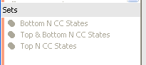
Then in the Coffee Chain database we create a set for the Top N States by Sum of Sales:2013-10-10 23_50_20-Tableau - sets from secondary

And here’s a view of that Coffee Chain data, where there are only 20 states:2013-10-10 23_51_46-Tableau - sets from secondary

But when we set up a view based on Superstore Sales and switch over to the Coffee Chain data, any and all sets are taboo greyed out:2013-10-11 00_02_28-Tableau - sets from secondary

However, we can use sets in calculated fields. The In/Out of a Set returns a boolean value, and here’s a simple formula used for the In Top N CC States calculated field:

IIF([Top N CC States],"In","Out")

This is treated as a dimension in the CoffeeChain data, which can lead to all sorts of applications, including using as a filter, color, or in additional calculated fields.

Note that in production, I’d probably use 1 and 0 as values instead of “In” and “Out” and then use aliases (because integers are faster than strings), and to solve a filter issue, however for this demo I’ll stick with In and Out to make it easier to understand and explain the filter issue further down.

Set from Secondary as Filter

Here’s a starting view from Superstore Sales as our primary data source:

Screen Shot 2013-10-26 at 11.11.44 AM

Before putting the In Top N CC States on the Filter Shelf, though, in the Coffee Chain data click on State as a linking field:

Screen Shot 2013-10-26 at 10.52.50 AM

Important note: whatever dimension(s) you use for the Set must be the blending dimension(s), no more and no less, if they are not then your results will be mighty strange. I’m still trying to work out what’s happening there. If you really need some calculation that blends on a different set of dimensions, then use a duplicated data connection for that blend.

Now you can drag the In Top N CC States calculated dimension from the Coffee Chain data onto the Filters Shelf, and here’s the filter setting:

Screen Shot 2013-10-26 at 10.52.20 AM

And the view:2013-10-11 00_06_11-Tableau - sets from secondary

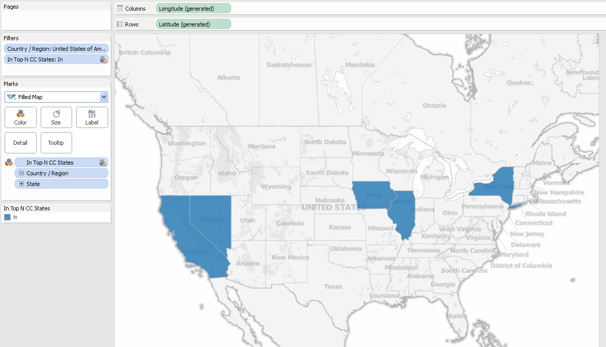
The worksheet is now only returning the 5 states from the primary and secondary data sources that meet the filter criteria from the set from the secondary data source. You’ve now used a Set from a secondary source!

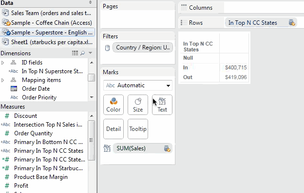
Set from Secondary on Color

How about using the set calculation in the view? If we change the In Top CC States to All values, and put a copy of the pill on the Color Shelf then we see three different values: In, Out, and Null.

Why are there Nulls? This is one aspect of data blending that can be confusing. In the Superstore Sales data, there are 49 US states (48 contiguous states plus the District of Columbia). In the Coffee Chain data, there are 20 states. 5 of those are In the Top N CC States set (blue above), 15 of those are Out (light orange). That leaves 29 states in the Superstore Sales data have no corresponding rows in Coffee Chain. For the In Top Top N CC States set calculation, rather than assigning those 29 states to In or Out, Tableau assigns a value of Null to those states because they don’t have corresponding values, and in this case they get a dark orange color. This is the same behavior Tableau has for any linked dimension value from the secondary that doesn’t have corresponding values in the primary.

How can we help those Nulls come Out of the closet become part of the Out of the set?

This assignment of Null values is done in the primary data source, as there’s so way we can change it in the secondary (without doing some sort of padding in the secondary for all of those states). However, there is a way we can do that in the primary data source. Tableau does all the computation it can within each data source, then blends the data sources together, at which point things like calculations that refer to another data source are computed. We can create a calculation in the primary that refers to the set in the secondary, and test whether the set calculation is returning Null. Here’s the formula from Superstore Sales for the Primary In Top N CC States calculated field:

IFNULL(MIN(IIF([Sample - Coffee Chain (Access)].[Top N CC States],"In","Out")),"Out")

The inner IIF() is a row-level calculation that evaluates the In/Out of the Set, then that gets wrapped in MIN() because we’re working across the blend – Tableau requires us to aggregate all measures and dimensions used in calculated fields from other data sources. The IFNULL() then tests the result of the MIN(), and if there’s a Null from one of those 29 states that is in the primary but not the secondary, the IFNULL() Outs that one as well. Here’s a view with the calculation, where now everything is In or Out:2013-10-11 00_27_02-Tableau - sets from secondary

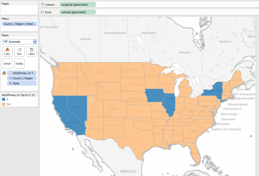
But you don’t have to be monogamous limit yourself to just one set. You can use combined sets from the secondary, for example in this view with CoffeeChain as the Primary I’m showing the top and bottom 5 states from the CoffeeChain data: 2013-10-11 00_35_02-Tableau - sets from secondary

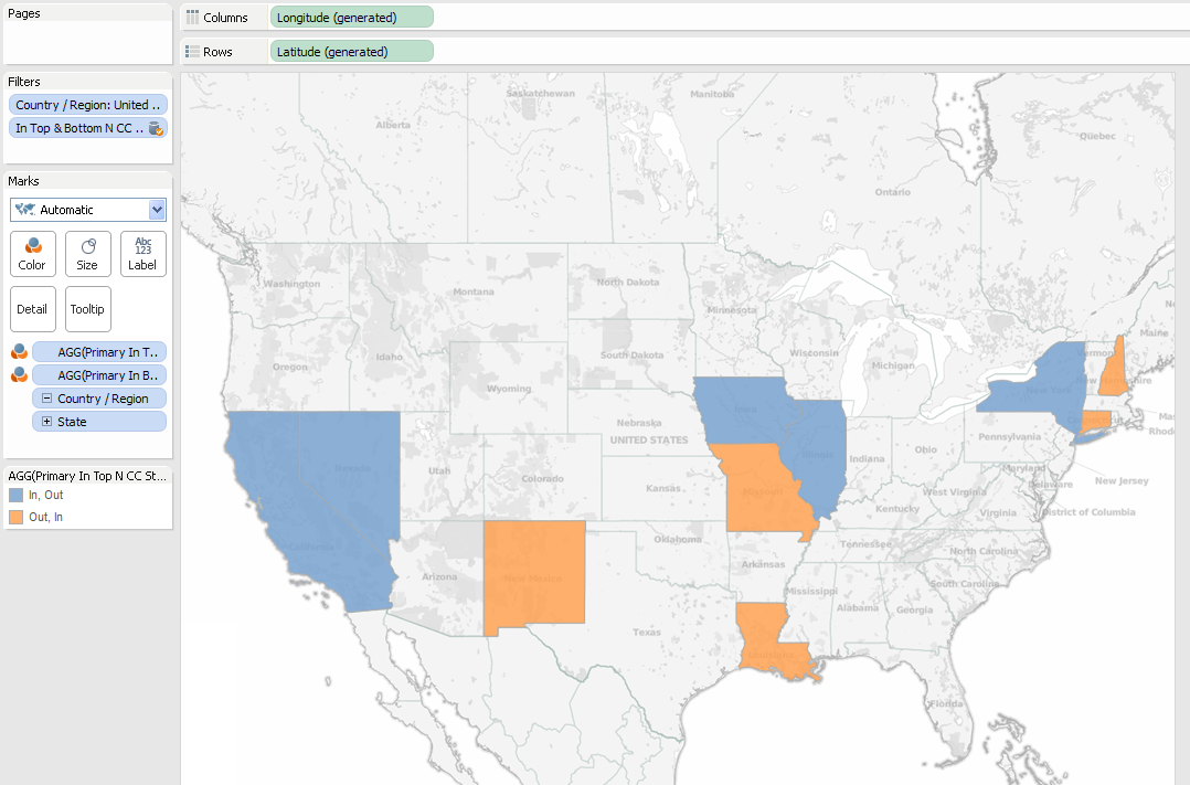
Now to talk about complications and workarounds before getting into some advanced cases:

Discrete vs. Continuous Measures

It’s important to note that the Primary In Top N CC States set calculation is a measure, because it’s using an aggregate from the secondary data source. 2013-10-11 00_38_12-Tableau - sets from secondary

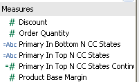
One effect is that Tableau won’t let us filter on discrete (blue) measures like the Primary In Top N CC States:

2014-01-30 17_59_48

My understanding is that this has to do with Tableau needing to know the domain (range of values) of measures to build the filter. (Here’s a Tableau Idea to support this, vote it up!) However, we can filter on continuous measures, so if you want to use that primary filter you can change the calc to return numbers instead of strings, like this calc called Primary In Top N CC States Continuous:

IFNULL(MIN(IIF([Sample - Coffee Chain (Access)].[Top N CC States],1,0)),0)

And this will work fine as a filter:

2014-01-30 18_07_01

Alternatively, you could use a table calc filter such as LOOKUP([Primary In Top N CC States],0) since discrete measures based on table calculations can be used as filters. I prefer the regular aggregate for performance reasons: Table calculation filters are applied after the data has been returned to Tableau, so that can lead to a lot of unnecessary traffic across the wire.

Using In/Out of Secondary Set in Primary Crosstab

In a simple view in Coffee Chain and our Top N set, we can quickly see the Sum of Sales for the In/Out of the set: 2013-10-11 00_46_08-Tableau - sets from secondary

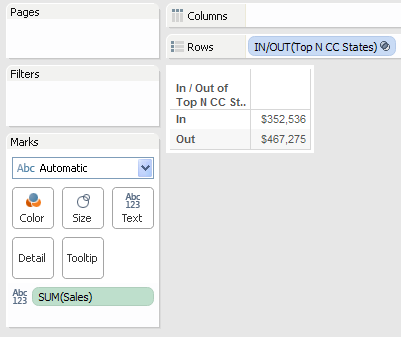
We can even set that up from the Superstore as Primary, using the In Top N CC States set calculation from the Coffee Chain secondary, all we need to do is make sure that State is turned on as a blending field and do a little extra filtering to get rid of those pesky Null values:2013-10-11 00_51_13-Tableau - sets from secondary


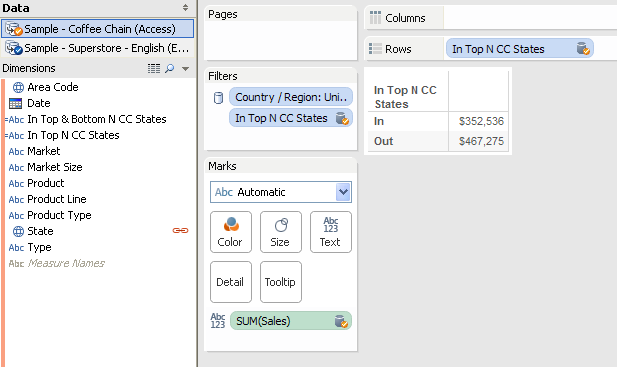
Advanced Uses for Secondary Sets

You can mix and match Sets from Primary and Secondary sources, here are three examples:

Cohort Analysis

In this view,  we’re looking at trends for profits broken down by the performance reviews of our sales people, looking to see if there are any trends. The sales data comes from Superstore Sales, the performance reviews are coming from a secondary data source. The panes are created by the In/Out of the Top 40 Customers by Profit. The top pane shows the sales for the Top 40 customers, the bottom pane everyone else. The lines are colored by the In/Out of the Top 5 Salespeople:

Screen Shot 2014-01-30 at 6.31.38 PM


Combining Sets Across Data Sources

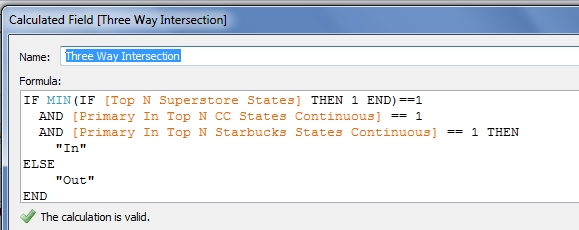
To create a combined set, we can use a calculated field that evaluates the sets from the different data sources, like this one that gets the intersection of the Top N States for Sales from both Superstore Sales and Coffee Chain, assuming the Superstore Sales is primary:

Screen Shot 2014-01-30 at 6.36.59 PM


And here it is used in a view, with the Top 5 States from each, only 3 states overlap:
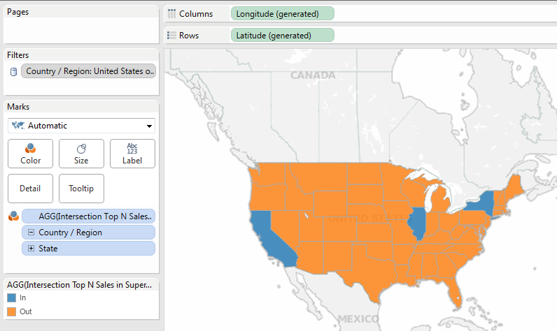
Screen Shot 2014-01-30 at 6.37.32 PM


The Three Way

Why stop at only two sets from different data sources? In this view using Coffee Chain as primary, we’re coloring the states based on the In/Out of the Top N States by Coffee Chain Sales, the Top N States with highest # of Starbucks per capita (data from Statemaster.com), and Top N States by Superstore Sales. Three data sources, three sets:

Screen Shot 2014-01-30 at 6.45.24 PM

And, of course, you can build calculated fields as well, here’s one in Superstore:

Screen Shot 2014-01-30 at 6.46.44 PM

Screen Shot 2014-01-30 at 6.48.00 PM


Conclusion

Here’s a link for the Tableau Public workbook for Sets with your Secondary.

With a little creativity and a whole lot of jokes at the maturity level of the average American teenage boy, we can get more out of data blending and sets. If you’d like Tableau to have more support for secondary sets out of the box (and generally treat secondary data sources more like primary data sources), please vote for http://community.tableausoftware.com/ideas/2773.

Now, go forth and use sets in strange places any position you want in new ways!

Orrery Remix – by Noah Salvaterra

When I first saw Jonathan Drummey’s Orrery post I sat there staring at it for a few minutes. Wow, right? So when the idea occurred to me to remix this classic I spent a few days wondering if I was serious. Once I managed to push my mouth closed I wondered if Tableau was the right tool for this job. Tableau, I thought, is just a tool for working with and visualizing existing data.

The Orrery is computation driven; the position of the planets are computed on the fly in Tableau and the data source driving this piece of art is almost an afterthought. It could literally have been built on Superstore Sales, you just need a place to hang the results of computations. In the case of Jonathan’s Orrery, this structure comes in the form of a SQL query that generates a hugely redundant data set. In all it has 51,840 rows. There are 18 planets (counting the sun and various moons), 360 ticks for the frames in the animation and 8 wedges for the slices that make up the pie charts used to draw each planet showing day and night (best use of pie charts ever!), 18 x 360 x 8 = 51,840.

I’m two blog posts deep into domain padding and using Tableau as a drawing engine, so I was reasonably sure the Orrery could be replicated with fewer rows in the source data, and that doing so could add flexibility in the number of ticks and the number of pie wedges. Improving the structure slightly didn’t seem significant enough on its own. I decided to give it a go if only for practice, and as an excuse to dive into understanding the original, but set two requirements that would need to be met prior to declaring it blog-worthy: First, Jonathan would have to be onboard, which he was. Second, it would need to bring something new to the table. I think I succeeded in finding an interesting point of view, but it isn’t exactly a new one…

Historical-Geocentric2

I’m going to put the earth back in the middle! 

My Orrery is built on two datasets. One that holds a single copy of the solar system data, and another for the intricate clockwork mechanism that makes it all tick. I connect these via data blending in Tableau. This blend could easily have been avoided, but it seemed like a more natural way to find the data. I figure this setup would make it easy to apply to other solar systems without duplicating effort. The planet data has 18 rows, taken from any of the 2,880 identical copies in Jonathan’s workbook (I used wedge 1 of tick 1, not that it matters), the mechanical structure has 72 rows. Since blending is a left join, I’d call this 72 rows total, but if you say 90, I guess I wouldn’t argue.

Now the domain padding isn’t that exciting. Well, sometimes it is, but I discussed it already in Creating data, multi-step recurrence relations, fractals and 3D imaging… without leaving Tableau. Nobody asked any questions on that yet, so I’ll assume it was all totally straightforward.

Since recreating the Orrery I’ve discussed my approach with Jonathan, and learned he considered using domain padding for the original, but ruled it out because of performance issues. Tableau 8.0 and 8.1 included some performance improvements for Table Calculations, so it is likely this approach only recently became feasible. Both techniques have strengths and weaknesses, it isn’t clear to me that one is better than the other.

There is one small point I can claim as a genuine improvement, that is changing the Days/Tick parameter from an integer to a float. Large values are needed to get satisfying movement from the slow moving outer planets, but some of the fast moving moons require less than one earth day per frame to see a smooth orbit.

Before I get any angry emails, I should mention that the planets don’t travel in perfect circles (or even ellipses), and that the solar system is also moving around the center of the galaxy and that it is all expanding from some infinitely dense singularity, which exploded for some reason. I’m not a physicist. This is more of a classroom model, a shiny one made mostly of brass. My interest is more on perspective than perfect accuracy. If I had a beta of Tableau 8.2, I might have shot for ellipses; in Windows, meh… close enough.

Venus Centered

Putting the earth in the middle is something I hadn’t seen a computer animation of. I knew the math could get complicated, which is why Copernicus and so many after preferred centering on the sun, but Tableau actually makes it pretty easy to change perspective. In fact, why just look at an earth centered solar system? What would it look like if we centered it on Venus or Mars? It turns out it is a lot crazier than I had imagined! Another surprise (though in retrospect it shouldn’t have been) is that from the perspective of slow moving outer planets the solar system model looks very similar to the sun centered view. I suppose this might develop over a longer time span than any I tried.

I started by taking perspective of standard heliocentric model, which is simplest math, both empirically and because I had Jonathan’s Orrery for reference. I then used a lookup table calculation so that the heliocentric position of the earth was visible to each of the other planets. Then, in what amounts to vector addition, I offset each planet by exactly the negative of the position of the earth. This puts the earth at the origin, and since an equal distance displaces each planet, the relative position is exactly the same in each frame. The history, on the other hand, traces out a very different path. A heuristic way to think of this, in terms of the clockwork orrery, is to pick the whole thing up by the earth, or some other planet, and holding that planet fixed while the mechanism, base and all continue spinning away as normal. Please don’t attempt this with your antique orrery, you will break it.

Optical iLLusion ~ Old or Young Lady ~ 02Trying to see things from two perspectives at the same time reminds me of optical illusions where you can see two possible pictures. With practice I can usually switch between perspectives quickly, but I can’t seem to see the old lady and the young lady at the same time. Why is that?

Since the trails give a historical record that is based on the center of the view, I thought it might be helpful to provide some landmark to compare it to another perspective. To accomplish this, I repeated this process of computing the position of a chosen planet to build a window that would dynamically remain centered. My original intent was that this window would follow the now moving sun, though again I found it interesting to approach with more generality, so the window can be centered on any planet or moon in the view. In any frame of the animation, the position of planets within these boxes is identical between the two models. Here is a video of simultaneous geocentric and heliocentric models:

Tube-train-in-motionI considered taking a shocking stand and arguing that the earth really is the center of the solar system, but the reality is that velocity is relative; for speed you need a fixed frame of reference. Imagine waking up on a train and seeing another train out the window that is travelling in the opposite direction. Both trains may be moving in opposite directions at 30 miles per hour, or just one train moving 60 miles per hour with the other standing stationary (or infinitely many other possibilities). To be absolutely certain of what is happening, the best approach is to look out of the window on other side. A stationary platform will clarify that your train is at rest and you’re about to miss your stop. When riding on a train, the earth is a fixed frame of reference from which we can discuss motion in an absolute context. The context determines the frame of reference, and generally this choice is so obvious you wouldn’t even realize you’re making it. When you consider planets, however, there is no handy universally agreeable point from which to gauge motion (at least not since Copernicus).

Often, regarding earth as a fixed point is preferable. Imagine trying to build a house or navigate to work while accounting for the spinning orbit of a planet that travels around the sun at 67,000 miles per hour. Most of us are unlikely to get further off this planet than an airplane ride, and planetary motion isn’t particularly relevant at that scale. Even taking a trip to the moon, my guess is that an accurate model of the solar system would be tremendous overkill. Any trip we take from our planet will begin with the same velocity and direction as the earth, and be subjected to the same gravitational forces for some time afterwards, so why does it even matter? Well, I think there is a deeper lesson in this story.

There is a famous quote of George Box, “Essentially, every model is wrong, but some are useful.” Finding out fundamental beliefs are wrong can be upsetting, or at least disorienting. Looking at the Venus centered solar system gives me some idea what it must have felt like for the first who pondered centering things on the sun. It also makes it easier to understand those who thought the idea was laughable.

Mathematical models are an important tool in science, including data science, but most models aren’t regarded as “the truth” until they are taken well out of their original context. I believe that as humans we are wired to search for the truths underlying our universe. I am anyway and there seems to be a strong historical case. But accepting mathematical models as such isn’t necessarily truth-ier than what came before. I do think the decrease in stake burnings is progress though.

The lesson here is one of complexity. I’m as guilty as the next guy of adding complexity to achieve a desired result, maybe more so. Something I’ve learned several times across several disciplines is that when you are adding layers to keep things working it is a good time to step back and check your assumptions. Changing your paradigm may result in something simpler, and while simplicity and truth are different things, they are both worth chasing.

So here is Orrery 2.0. Dynamic animation doesn’t work in Tableau public (currently) so please download for the full experience. Have fun experimenting with different centers and see some of the crazy orbits that evolve. Hopefully someone will enjoy this half as much as I did the original and a seed will be planted to push this even further. I can’t wait:

Download Orrery Workbook from Tableau Public

If you think my displacement approach is cheating and you’d like to go back to epicycles, or Ptolomey’s epicycles on epicycles (computers have come a long way since then, so this goes 5 epicycles deep), here is a Spiro-graph workbook to use as a starting point. The source dataset has only 2 rows; across 3 blog posts that brings my total to 6 workbooks, none of which has more than 100 rows in the source data. In fact, I believe that makes 106 rows altogether!


Download Spirograph Workbook from Tableau Public