Emily Kund’s identity crisis post resonated with a lot of people, me included, since as a new blogger I’m finding my voice and struggle with the same issues. “Super awesome data skills” are probably an advantage in this arena, but this is neither necessary nor sufficient to creating an interesting blog. I feel fortunate to have had several ideas that people have found interesting. These weird and wonderful creations have definitely pushed the envelope in terms of my abilities in Tableau. But after each post I think my next one should be something that can be applied to a business use case rather than dropping a workbook or four, however mind bending they may be.
After remixing Jonathan Drummey’s Orrery, I saw this tweet:

I printed it out and carried it around with me for a few days afterwards. I sincerely appreciate the complement. Often the things I’m most proud of and the things I am most complemented for are totally different, but this was a winner. The Orrery is sophisticated, no doubt, but hold on to your hat Andy… the death star is fully operational!
The survey in Emily’s post resulted in a pretty clear winner “Be the hippie you are and let it grow organically.” Not being that much of a hippie, I might paraphrase that as: write about something you find interesting and see where that goes. Fair enough. If you’re looking for techniques you can apply in the office tomorrow, look somewhere else. That isn’t what is happening here, that is SO not what is happening. No offense to such blogs, I’m a big fan of useful information and techniques and sincerely hope I can make my way in that direction at some point. But for now, I’m going to take the gloves off and embrace this niche, even if it means more headaches than sleep.
A quality I have that makes me a good data analyst is a talent for lateral thinking. I don’t know if this is something one is born with, or if it is a product of environment (or vaccinations). There are a few tricks I keep in the back of my mind, though, that can help kick this process along. When I notice everyone looking in one direction, I try to at least glance in the other. I’ve had some close calls crossing the street, but sometimes I see something that otherwise everyone would have missed. When this idea is applied to paradigms, every once in a while it can change everything.
Tableau is all about simple elegant approach to data visualization, yet my recent blog posts have been almost void of data and have used some heavy-duty techniques. Why? Well I don’t generally shy away from complexity, if anything I’m drawn to it. Not because I want to push it on others, just the opposite, but my experience is that sometimes the path to a simple story first leads through this crucible.
What would be a use case for Tableau that is furthest from what anyone intended? What if, instead of a simple, elegant, visual presentation Tableau was used to obscure, complicate, obfuscate, and confuse… rolling through synonyms in my head one jumped out at me. Enigma!
Tableau Enigma:
 1939. With the sound of bombs exploding in the distance and bullets whizzing nearby, a German soldier sits on a small folding stool. At first glance he appears to be typing a letter. Yet the typewriter has no paper in it, it doesn’t even have a place for it; instead 3 rows of lights arranged in the same configuration as the keyboard dot the top portion of the machine. Each time a key is pressed a light illuminates under a letter and is carefully recorded by a second man. When put this way it sounds a little crazy, but for one thing, the letter that lights up is NEVER the same as the key pressed and the carefully recorded letters appear to be complete gibberish. Actually, I’m not sure that helps. The typewriter is an Enigma machine, the pinnacle of World War II encryption technology and a key advantage for Germany in this war. Able to quickly and secretly communicate allowed them to coordinate their forces at a level never before seen. Though vastly outnumbered, this advantage might have won Germany the war, except for one thing. In Bletchley Park, a small village in central England, the code was broken.
I’d really love to wax historical on Enigma, but I’m a mathematician and an analyst. I can speak in a number of areas with authority, but history in not one of them. Hopefully someone with a solid background on this side and a rich flair for storytelling will fill in some of the details in the comments. I’m going to jump right in to a description of this odd contraption.
Overview:
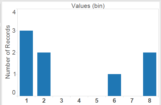
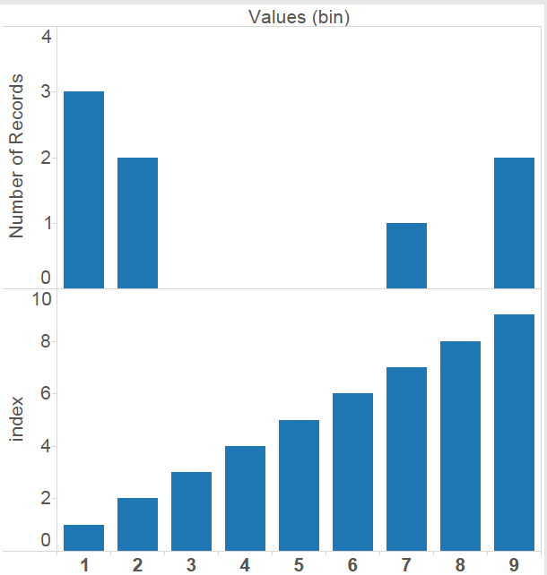
Enigma gets its strength from the interplay of mechanical and electrical systems, with batteries and light bulbs it is easy to create a machine that would do simple substitution encryption. But that type of code is also relatively easy to crack using letter frequencies. By coupling this technology with moving parts, basically an old timey cash register, a different substitution cypher is applied each time a key is pressed. So the same letter could be encoded to different letters, for example AAAAAAA could be encoded as PFQDVKUEKE. Likewise, different letters could be encoded to the same one; that is PFQDVKUEKE could be encoded as AAAAAAAAAA. These examples were created with the Enigma workbook and demonstrate a convenient property of Enigma: it is self-reciprocal. Encryption and Decryption are the same process, so decoding an encrypted message only required the machine be set up in the same way as the encryption machine. These setup instructions were very important to the whole operation; generally these settings were distributed monthly, with different setup for each day. This meant that even if an Enigma machine and setup instructions were captured, it wouldn’t represent a security breach for more than a few weeks. Technically, the daily settings were meant to be used only for transmitting randomly chosen setup instructions which would be used once then discarded. Had this been done consistently it might not have been possible to break. Operator error played a key role in the weakness of the Enigma cipher.
Mechanical:
 A basic, early WWII military enigma comes with 5 interchangeable rotors, labeled I, II, III, IV, V. Three of these rotors are selected and placed inside the machine in left, middle and right positions, based on the daily settings. Each rotor is labeled around its circumference with the letters of the alphabet (or the numbers 1-26). The rotor fits into its chosen location in 26 ways, recorded in the daily settings as the letter in the top position. Each time a key is pressed the right rotor moves forward one step. Each rotor has a fixed notch on it, which causes the adjacent rotor to advance as the notch passes the top position. Mechanically, this is like an odometer, but instead of turning over at zero each wheel has a different point. Royal flags waive kings above is a mnemonic used at Bletchley Park for this; it has a notch at R, II at F, III at W, etc. The middle wheel notch similarly steps the left most wheel forward. So the right wheel moves fastest, the middle wheel moves once every 26 letters and the left most wheel moves once every 26^2=676 letters. In practice Enigma messages were limited to 250 characters, with longer messages being sent in pieces.
Electrical:
When a key is pressed, the mechanism takes one step, and a circuit is subsequently completed. This causes a light to illuminate under the corresponding encoded (or decoded) letter.
 The current passes through each of the rotors from right to left and then back again. Each rotor contains a jumble of wires in a predetermined configuration. Since the rotors move with each key press, the position at which the current enters and the letter presently in that position both play a role in the encryption. After passing through right, middle, then left rotor in that order, the current flows through a fixed single sided rotor called a reflector (or some equivalent term in German). The reflector directs the current back in the opposite direction, from left to right, applying the inverse permutation.
Military enigma machines also included a plug board on the front where 10 sets of wires could be plugged in.  Each wire enacts a simple swap of 2 letters both in the forward and backward direction, so if A&B are connected then A is sent through the upper machine as B. If it comes out of the upper machine as Y and Y & Z are also connected then it will show as Z on the light board.
Enigma Difficulties:
The calculations for Enigma are a complicated web, not just with nesting, but also with branching. It is like an Orrery with electricity flowing through it. Each attempt I made at Enigma came to a grinding halt before the finish line. At one point, editing a calculation took as long as 5 hours. Note that isn’t refreshing the Viz, just typing into calculations with auto-updates turned off, before I even hit OK! Refreshing the worksheet also took hours, so it didn’t seem like Enigma would make it to Tableau public or a blog post, but by that point I just wanted to finish it.
Tableau has a built in equation checker for calculations; if you create your own calculated fields then you’ve probably seen some feedback from this feature just below your calculation on the left, usually in the form of a green checkmark (yay!) or a red x (boo!). I suspected this might be the source of the issue, since it must be parsing through all the nesting in order to check for things like circular references. Circular references and mixing aggregates with non-aggregates are my most common reason for getting an x, and usually I appreciate this feature; it protects me from myself. But when your workbook freezes for hours at a time, it really gives you time to think. Things like, “Is there a way to turn the equation checker off?” and “When was the last time I saved?” were among my favorites. Eventually I decided to reach out for some help with this and mailed my mess of a workbook to Zen Master Joe Mako.
Joe is an expert in most areas of Tableau; he is so good that I’ve speculated that Tableau has a Zen Master setting buried in some menu where nobody else has ever looked. That said there are a couple areas where even Joe calls on someone else. In this case, that person was Zen Master Richard Leeke. At this point the Enigma is as much his as it is mine. I lost count of how many times we passed this back and forth, with several iterations taking place before we had it doing much of anything.
There were a lot of calculations taking place, compared to most Tableau workbooks, but neither Richard nor I could come up with a solid theory why it would take hours to encode a 10-character message (my test message was “HELLOWORLD”). Richard had found table calculations to be the source of such slowdowns in the past, and helped to improve these in recent Tableau releases (Thanks!). His initial analysis of the Enigma workbook showed a lot of time going into these, so that was where we started. The data for Enigma comes primarily from user input, so like several of my other posts I started with a very small dataset, 2 rows small. Using data densification I made a general array structure over which the necessary calculations take place. That means table calcs appear at a very low level, and everything is built on top of that, so it made sense that a problem there could be making the whole thing drag. So I replaced the array structure with a hard coded data source. In practice, Enigma messages were generally limited to 250 characters, so this compromise didn’t raise any concerns in terms of historical accuracy. But it was still slow.
The next use of table calculations was to count the number of times the notch passed the top position on the right and middle rotors; basically I had a notch indicator (based on the rotor position) which was used in a running sum. Thinking through this calculation, and carefully working through various cases, I realized that it was again something I could do without using table calcs, just a little more algebra required on my part. So all table calculations gone, still slow (and not even working yet).
The next thing we thought about was the branching case statement I had used for the scrambling that takes place on each of the rotors. It was a long case statement first on the rotor selection then the current position of that rotor (so basically 5*26=130 if-else statements). This naïve approach on my part turned out to be the main source of slowdown. One idea I had from the start was to use blending somehow for the rotors, rotating the blending field to correspond with the physical position in a physical Enigma, I just wasn’t sure I could make blending work in this way. Luckily Richard came up with a simpler blending solution. The rotor datasources just contain a field for the rotor selection and one for the character substitution (in each direction). A 26 letter string for the permutation was a much cleaner way to state the permutation; for example rotor I is “EKMFLGDQVZNTOWYHXUSPAIBRCJ”. Understanding Enigma means going back and forth between the letters A-Z and the numbers 1-26 a few times (A1, B2, … Z26). I had converted the numbers to characters at the start, so I could make use of modular arithmetic, but not wanting to add overhead from type conversions, I hadn’t used them in the middle. The string above is a very simple representation of a permutation, A->E, B->K, C->M, …, Z->J, made even better because the input letter was represented in numerical form, i.e. for the string above, mid(string,1,1)=E, mid(string,2,1)=K, mid(string,3,1)=M, …, mid(string, 26,1)=J. These characters could then be converted back to numbers. Now you may wonder why blend this at all, isn’t it simpler to put these values into a calculation? I think it is, but there seems to be a significant performance difference between the two approaches. In the corner case of this workbook, that difference (along with the simplification of the permutations) took the refresh time from more than 2 hours to under a second. Blazing fast. Just one problem: it still didn’t work.
 The speed improvement was based on the part that worked, but it was throwing an error before it was finished. There were only about 55 or so interconnected calculations at this point, but many of these were used more than once. The image on the left is a zoomed out view of the complex calculation call-tree that Richard built to understand this nesting. Having solved the width problem, there was now one with depth. Richard built a simple workbook to explore the issue and found a curious limitation, one I expect doesn’t get hit very often, but it seems that calculations can be no more than 128 levels deep. So f1(f2(f3(…f128(x)…))) more than that and you’re out of luck (for now). If you’re computing 128 levels deep though, chances are there is some room for improvement, and that was the case here. At this point, Enigma was trying to do around 136. I had used a separate calculation for each of the 10 wires in the forward direction, then another for each of the 10 wires on the way back. So that was 20 calculations that could be done in 2. I’d have made this simplification earlier, but clearly this wasn’t the source of the slowdown and when changing a calculation takes half a day it is hard to think about such things.
I strutted around for a day or two before I realized another problem. I had created a working Enigma machine in Tableau, that was historically accurate in terms of its functionality, but that doesn’t make for a very interesting Tableau blog. I was going to need a Viz.
The Viz:
 The Enigma machine is literally a black box. Not much to look at. My first inclination for an Enigma viz was something that looked like an Enigma machine. With an Enigma as background image I planned to highlight the input key and the output light with circles. As each rotor turns, the operator can see the letter currently in the top position through a small window. Two circles and three letters, easy, they wouldn’t even need to be on the same worksheet. Flipping through these using the pages shelf and you might get a sense of looking over the shoulder of an Enigma operator, but it still didn’t seem very illuminating. Complexity of execution isn’t my goal; it just seems like an awful lot of wasted potential. Still thinking along these lines, I considered using 26 separate background images for fingers hitting keys. That would be a fun view, but downloading 26 images would probably make the viz very slow to load and I wanted to do something on Tableau Public. Custom mark types for hands might be a suitable work around, but it definitely seems like more flash than substance. I decided against a photo realistic Enigma or even a stylized view from the outside. Could Tableau tell the story of what is happening INSIDE the Enigma machine? I found one such visualization on the web, but creating it would mean building quite a bit of visualization structure on top of what was probably already my most sophisticated tableau workbook.
I wanted arrows that would mark the input and output letters, plus rotating ones to show the notches on the turning wheels. The path through the machine would need to be shown as a series of lines. A box could be used to mark the top letters, visible to the operator. Also, letters around the inside and outside each rotor would have to move dynamically in each frame. Oh, and it is all interconnected, so it needs to be done in one viz. Gulp. With that goal in mind, I built my first inside-out version. It took about 2 minutes to load. Thus began another chain of emails with Richard Leeke. The main improvement from that round actually added a table calculation, by using previous value the message only needed to be computed once, rather than for each of the 320 points I allowed for in the Viz. It seems to be consistently between 8 and 12 seconds for me now, so please be patient and use this time to consider that it is more than 99.93% faster than the first attempt. I had a slightly prettier version that used a dual-dual axis, but also was slowing things down, so it is a single line plot now. Note, my original dashboard was too wide for a blog post, so I rotated it clockwise by 90 degrees (i.e. the Right rotor is on the bottom). Anyway, Tableau Enigma, please enjoy:
Here is a link to the Enigma workbook on Tableau Public.
Conclusion:
I think maybe Emily’s survey was missing an important option. Collaborate! We’ve all got strengths and weaknesses and finding people who can lift you when you’re stuck is the easiest way to increase your impact. Bring something to the table and it will be worth their while. I’m glad I’ve got some people like that and hope they have as much fun as I do. Thanks again to all those who helped with this.
Final note:
Though I sang the praises of two Zen Masters in this post, there is one that hasn’t gotten a mention here who probably should. Jonathan Drummey is a genius and has been a great help to me in advancing my Tableau skills not to mention my blogging ones. I have little doubt Jonathan could add something awesome here, maybe he still will, but I’ve kept this project a secret. I realized that if I dropped a completed Enigma on Jonathan it would blow his mind clear across the room. His Orrery had that effect on me, but the fuse burned for a few months before the explosion. Thanks Jonathan!